library(tidyverse)
library(janitor)
library(forcats)
library(purrr)
library(readxl)
library(gt)
library(lubridate)Packages
The data
The toy data set is captured in an Excel file, which can be downloaded from my Github page. This small data set contains data for 10 persons across nine variables: Person ID, Date of birth, Gender, Nationality, Question 1, Question 2, Question 3, Question 4, and Question 5. Below is a screenshot of the data.
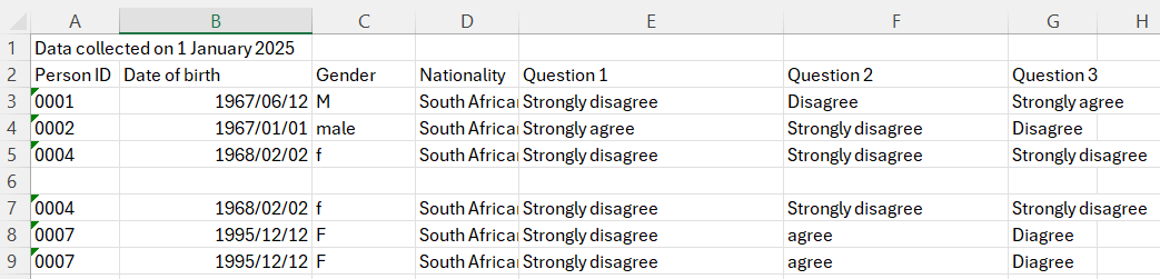
There are several problems with this data set:
The variable names are not in the first row
The variable names start with capitals and contain spaces
The rows of persons 0004 and 0007 are duplicated
In the Gender column we find four codes, i.e. M, F, male and f
In the Question 1 column we find that “Agree” had been incorreclty typed as “agree”
In the Question 5 column we find that “Disagree” has been incorrectly typed as “Diagree”
Row 8 of the data set is completely empty
The Nationality column is a constant (all the entries are the same) and therefore carries no useful information
We really want the data for Question 1 to Question 5 to be numeric rather than text.
Whereas it is relatively easy to detect and correct such problems in a small data set, it can become very difficult and tedious with a large data set. Moreover, cleaning the data in the Excel file will not leave an explicit record of what has been done to the original data set, which might compromise the reproducibility of the entire data analysis process. It is usually better to leave the original Excel file intact and to then clean up the data in R, where all the steps that were taken can be saved in a script file.
Importing the data and cleaning the column names
dirty_data <- read_excel("dirty_data.xlsx")

names(dirty_data)
[1] "Data collected on 1 January 2025" "...2"
[3] "...3" "...4"
[5] "...5" "...6"
[7] "...7" dirty_data %>%
gt()| Data collected on 1 January 2025 | ...2 | ...3 | ...4 | ...5 | ...6 | ...7 |
|---|---|---|---|---|---|---|
| Person ID | Date of birth | Gender | Nationality | Question 1 | Question 2 | Question 3 |
| 0001 | 24635 | M | South African | Strongly disagree | Disagree | Strongly agree |
| 0002 | 24473 | male | South African | Strongly agree | Strongly disagree | Disagree |
| 0004 | 24870 | f | South African | Strongly disagree | Strongly disagree | Strongly disagree |
| NA | NA | NA | NA | NA | NA | NA |
| 0004 | 24870 | f | South African | Strongly disagree | Strongly disagree | Strongly disagree |
| 0007 | 35045 | F | South African | Strongly disagree | agree | Diagree |
| 0007 | 35045 | F | South African | Strongly disagree | agree | Diagree |
Inspection of the dirty_data data frame shows that the first row of the Excel file produced incorrect column names. The proper column names are now located in the first row of the data frame. By instructing R that the column names are in the first row of the data frame we can solve this problem.
dirty_data <- dirty_data %>%
row_to_names(row_number = 1)
glimpse(dirty_data)Rows: 7
Columns: 7
$ `Person ID` <chr> "0001", "0002", "0004", NA, "0004", "0007", "0007"
$ `Date of birth` <chr> "24635", "24473", "24870", NA, "24870", "35045", "3504…
$ Gender <chr> "M", "male", "f", NA, "f", "F", "F"
$ Nationality <chr> "South African", "South African", "South African", NA,…
$ `Question 1` <chr> "Strongly disagree", "Strongly agree", "Strongly disag…
$ `Question 2` <chr> "Disagree", "Strongly disagree", "Strongly disagree", …
$ `Question 3` <chr> "Strongly agree", "Disagree", "Strongly disagree", NA,…dirty_data %>%
gt()| Person ID | Date of birth | Gender | Nationality | Question 1 | Question 2 | Question 3 |
|---|---|---|---|---|---|---|
| 0001 | 24635 | M | South African | Strongly disagree | Disagree | Strongly agree |
| 0002 | 24473 | male | South African | Strongly agree | Strongly disagree | Disagree |
| 0004 | 24870 | f | South African | Strongly disagree | Strongly disagree | Strongly disagree |
| NA | NA | NA | NA | NA | NA | NA |
| 0004 | 24870 | f | South African | Strongly disagree | Strongly disagree | Strongly disagree |
| 0007 | 35045 | F | South African | Strongly disagree | agree | Diagree |
| 0007 | 35045 | F | South African | Strongly disagree | agree | Diagree |
However, some problems with the column names remain. In particular, the column names start with upper case letters, which is considered bad practice. In addition, several column names contain spaces, which is also considered bad practice. These problems can be solved with the clean_names() function of the janitor package.
dirty_data <- dirty_data %>%
clean_names()
glimpse(dirty_data)Rows: 7
Columns: 7
$ person_id <chr> "0001", "0002", "0004", NA, "0004", "0007", "0007"
$ date_of_birth <chr> "24635", "24473", "24870", NA, "24870", "35045", "35045"
$ gender <chr> "M", "male", "f", NA, "f", "F", "F"
$ nationality <chr> "South African", "South African", "South African", NA, "…
$ question_1 <chr> "Strongly disagree", "Strongly agree", "Strongly disagre…
$ question_2 <chr> "Disagree", "Strongly disagree", "Strongly disagree", NA…
$ question_3 <chr> "Strongly agree", "Disagree", "Strongly disagree", NA, "…dirty_data %>%
gt()| person_id | date_of_birth | gender | nationality | question_1 | question_2 | question_3 |
|---|---|---|---|---|---|---|
| 0001 | 24635 | M | South African | Strongly disagree | Disagree | Strongly agree |
| 0002 | 24473 | male | South African | Strongly agree | Strongly disagree | Disagree |
| 0004 | 24870 | f | South African | Strongly disagree | Strongly disagree | Strongly disagree |
| NA | NA | NA | NA | NA | NA | NA |
| 0004 | 24870 | f | South African | Strongly disagree | Strongly disagree | Strongly disagree |
| 0007 | 35045 | F | South African | Strongly disagree | agree | Diagree |
| 0007 | 35045 | F | South African | Strongly disagree | agree | Diagree |
All the variable names now start with lower case letters and the empty spaces have been replaced by underscores.
Remove empty and duplicate rows and constant columns from the data frame
We employ the remove_empty() function of the janitor package to remove empty rows.
dirty_data <- dirty_data %>%
remove_empty() %>%
distinct() %>%
remove_constant()value for "which" not specified, defaulting to c("rows", "cols")dirty_data %>%
gt()| person_id | date_of_birth | gender | question_1 | question_2 | question_3 |
|---|---|---|---|---|---|
| 0001 | 24635 | M | Strongly disagree | Disagree | Strongly agree |
| 0002 | 24473 | male | Strongly agree | Strongly disagree | Disagree |
| 0004 | 24870 | f | Strongly disagree | Strongly disagree | Strongly disagree |
| 0007 | 35045 | F | Strongly disagree | agree | Diagree |
The empty row, the duplicate rows and the Nationality column (which was a constant) have been removed.
Fixing the date of birth column
The Excel date column was incorrectly imported. We fix this with the convert_to_date() function of the janitor package.
dirty_data$date_of_birth <- convert_to_date(dirty_data$date_of_birth)
dirty_data %>%
gt()| person_id | date_of_birth | gender | question_1 | question_2 | question_3 |
|---|---|---|---|---|---|
| 0001 | 1967-06-12 | M | Strongly disagree | Disagree | Strongly agree |
| 0002 | 1967-01-01 | male | Strongly agree | Strongly disagree | Disagree |
| 0004 | 1968-02-02 | f | Strongly disagree | Strongly disagree | Strongly disagree |
| 0007 | 1995-12-12 | F | Strongly disagree | agree | Diagree |
Calculating current age and adding it as a variable
dirty_data$age <- as.period(interval(start = dirty_data$date_of_birth,
end = ymd("2025-01-01")),
unit = "years")
dirty_data$age <- dirty_data$age@year
dirty_data %>%
gt()| person_id | date_of_birth | gender | question_1 | question_2 | question_3 | age |
|---|---|---|---|---|---|---|
| 0001 | 1967-06-12 | M | Strongly disagree | Disagree | Strongly agree | 57 |
| 0002 | 1967-01-01 | male | Strongly agree | Strongly disagree | Disagree | 58 |
| 0004 | 1968-02-02 | f | Strongly disagree | Strongly disagree | Strongly disagree | 56 |
| 0007 | 1995-12-12 | F | Strongly disagree | agree | Diagree | 29 |
Storing a variable as a factor
dirty_data <- dirty_data %>%
mutate(gender = as.factor(gender))
glimpse(dirty_data)Rows: 4
Columns: 7
$ person_id <chr> "0001", "0002", "0004", "0007"
$ date_of_birth <date> 1967-06-12, 1967-01-01, 1968-02-02, 1995-12-12
$ gender <fct> M, male, f, F
$ question_1 <chr> "Strongly disagree", "Strongly agree", "Strongly disagre…
$ question_2 <chr> "Disagree", "Strongly disagree", "Strongly disagree", "…
$ question_3 <chr> "Strongly agree", "Disagree", "Strongly disagree", "Diag…
$ age <dbl> 57, 58, 56, 29dirty_data %>%
gt()| person_id | date_of_birth | gender | question_1 | question_2 | question_3 | age |
|---|---|---|---|---|---|---|
| 0001 | 1967-06-12 | M | Strongly disagree | Disagree | Strongly agree | 57 |
| 0002 | 1967-01-01 | male | Strongly agree | Strongly disagree | Disagree | 58 |
| 0004 | 1968-02-02 | f | Strongly disagree | Strongly disagree | Strongly disagree | 56 |
| 0007 | 1995-12-12 | F | Strongly disagree | agree | Diagree | 29 |
Checking the unique levels of a factor and recoding the levels of a factor
The unique() function shows that there are four levels in the gender column (i.e. f, F, M and male), where only two were expected (i.e. F and M).
We use the mutate() function of the dplyr package along with the fct_recode() function of the forcats package to recode the gender factor such that f becomes F and male becomes M.
unique(dirty_data$gender) [1] M male f F
Levels: f F M male### Recode the levels of a factor
dirty_data <- dirty_data %>%
mutate(gender = fct_recode(gender, F = "f", M = "male"))
unique(dirty_data$gender)[1] M F
Levels: F Mdirty_data %>%
gt()| person_id | date_of_birth | gender | question_1 | question_2 | question_3 | age |
|---|---|---|---|---|---|---|
| 0001 | 1967-06-12 | M | Strongly disagree | Disagree | Strongly agree | 57 |
| 0002 | 1967-01-01 | M | Strongly agree | Strongly disagree | Disagree | 58 |
| 0004 | 1968-02-02 | F | Strongly disagree | Strongly disagree | Strongly disagree | 56 |
| 0007 | 1995-12-12 | F | Strongly disagree | agree | Diagree | 29 |
Check the unique levels of item responses
To identify the unique levels in the item responses we first use the select() function of the dplyr package to select the columns containing the items. Next we use the map() function of the purrr package to find the unique levels. Results show that there are seven levels, i.e. (a) Strongly disagree, (b) Strongly agree, (c) Disagree, (d) agree, (e) Agree, (f) NA, and (g) Diagree. It is clear that “agree” and “Diagree” represent typing errors.
unique_levels <- dirty_data %>%
select(question_1:question_3) %>%
map(unique) %>%
unlist() %>%
unique()
print(unique_levels)[1] "Strongly disagree" "Strongly agree" "Disagree"
[4] "agree" "Diagree" Converting the items to numeric variables
To convert the item responses to numbers we employ the mutate(), across() and case_when() functions. We type each possible level and assign a number to that level. Note that “Disagree” and “Diagree” were both assigned the number 2, while “Agree” and “agree” were both assigned the number 3.
dirty_data <- dirty_data %>%
mutate(across(question_1:question_3, ~ case_when(
. == "Strongly disagree" ~ 1,
. == "Disagree" ~ 2,
. == "Diagree" ~ 2,
. == "Agree" ~ 3,
. == "agree" ~ 3,
. == "Strongly agree" ~ 4,
TRUE ~ NA_real_ # Handle any unexpected values
)))
dirty_data %>%
gt()| person_id | date_of_birth | gender | question_1 | question_2 | question_3 | age |
|---|---|---|---|---|---|---|
| 0001 | 1967-06-12 | M | 1 | 2 | 4 | 57 |
| 0002 | 1967-01-01 | M | 4 | 1 | 2 | 58 |
| 0004 | 1968-02-02 | F | 1 | 1 | 1 | 56 |
| 0007 | 1995-12-12 | F | 1 | 3 | 2 | 29 |