Exploratory factor analysis of the Big Five Inventory: Walkthrough with the psych pagackage

R
exploratory factor analysis
Author
Affiliation

Deon de Bruin

Department of Industrial Psychology, Stellenbosch University

Published

January 21, 2025

Exploratory factor analysis

Exploratory factor analysis (EFA) is a statistical technique that researchers use to find the latent structure underlying a set of manifest variables. In the context of scale development and validation EFA is typically used to (a) identify the number of factors (latent variables) that underlie a set of scale items, and (b) identify the items that are the best and worst indicators of the factors. With respect to the latter, the best items are typically those that have a salient relationship with one and only one factor. The worst items may come in two varieties. First, they are items that do not have a salient relationship with any of the factors, or second, they are have salient relationships with two or more factors.

For instance, we might expect (a) that an EFA of the Big Five inventory will show that five major factors underlie the 25 items, and (b) that each of the say, Extroversion items, have a salient relationship with one and only one factor (and the same applies for the Neuroticism, Conscientiousness, Agreeableness, and Openness items). A result that corresponds with this structure will give us confidence that the items are actually measuring the constructs they are intended to measure. By contrast, a result that produces more than five major factors or one that shows that some items fail to have a salient relationship with any of the factors, or one that shows that items have salient relationships with the “wrong” factors, will indicate that the items are not operating as expected.

How is this different from confirmatory factor analysis?

A confirmatory factor analysis (CFA) of the Big Five Inventory would start with an explicit measurement model where the number of factors are fixed at five and where each item is allowed to have a direct relationship with one and only one factor. For instance, all the Extroversion items will be specified to have a direct relationship with the Extroversion factor, but no direct relationships with the remaining factors, and so on. Here the task of the factor analysis is typically to (a) examine how well this pre-defined structure (or measurement model) fits observed data, (b) to estimate the strength of the relations between the items and the factors, and (c) to estimate the strength of the relations between the factors. Good fit will give us confidence that the items are functioning as expected, whereas poor fit will indicate that the measurement model may need to be revised.

By contrast, an EFA is less restrictive (it is also sometimes referred to as unrestricted factor analysis). First, rather than forcing a predetermined number of factors on the data, the analyst will allow the data itself to suggest the number of factors to “extract” or retain. Second, in an EFA all items are typically allowed to have relationships with all the factors. Again, the analyst will allow the data to reveal which items have strong relationships with which factors.

In practice, an EFA is seldom done in a pure exploratory fashion. In most case it is likely that the analyst will have ideas of (a) how many factors to expect and (b) which items are likely to have strong relationships with which factors. This is so because psychological tests and scales are typically developed to reflect a theoretical structure, where the developers know what latent variables they want to measure and the items are explicitly written to reflect those latent variables.

Exploratory factor analysis and the development of the Big Five model of personality

The development of the Big Five model of personality actually is a very good example of how exploratory factor analysis was used in a true exploratory fashion to discover (without a pre-determined theory or model) what the basic dimensions of personality are. This line of research is based on the so-called “lexical hypothesis”, which holds that if a personality attribute is important, there will be a word in the lexicon to describe it. Much of this work focused on adjectives, such as “friendly”, “aggressive”, “scatter-minded”, “lazy”, “nervous”, “humorous”, “ambitious”, and so on.

Across many different languages, countries and cultures researchers have discovered (using the technique of EFA) that ratings of people’s personality attributes (as reflected by such adjectives as listed above) typically yielded five major latent variables (or factors).

In practice, these types of studies identify large numbers of adjectives that would be representative of the lexicon of personality descriptors. Next, the researcher(s) ask large numbers of people to rate themselves (or sometimes other people) on each of the adjectives. These ratings typically focus on how well the adjective describes the person and could, for instance, be done using an ordinal rating format (e.g. 1 = Not like me at all, 2 = A bit like me, 3 = Like me, and 4 = Very much like me), or a binary format (1= No and 2 = Yes). EFA is then performed on these ratings and the goal is to allow the data to reveal (a) the number of latent variables or factors that underlie these adjectives, and (b) the nature or meaning of the factors. The latter is accomplished by inspecting the particular adjectives that have strong relationships with the various factors. In this way, EFA was used to “discover” (without restrictions) that across languages, countries and cultures, the lexicon describing personality attributes can be reduced to five major factors, and that these factors could be labeled as Extroversion, Neuroticism or Stability, Agreeableness, Conscientiousness, and Openness or Intellect.

Many different personality inventories and scales of the Big Five factors have been developed on the basis of this corpus of exploratory factor analyses . The Big Five Inventory is one such scale. Note that the scale was explicitly developed to measure the Big Five factors and that the items were carefully selected to serve as indicators of these factors. An EFA of the Big Five Inventory takes place against the background of this knowledge. Whereas the EFA will be done without (too many) restrictions, the analysis is not entirely exploratory.

The packages

library(psychTools)
library(psych)
library(GPArotation)

Attaching package: 'GPArotation'
The following objects are masked from 'package:psych':

    equamax, varimin
library(tidyverse)
── Attaching core tidyverse packages ──────────────────────── tidyverse 2.0.0 ──
✔ dplyr     1.1.4     ✔ readr     2.1.5
✔ forcats   1.0.0     ✔ stringr   1.5.1
✔ ggplot2   3.5.1     ✔ tibble    3.2.1
✔ lubridate 1.9.4     ✔ tidyr     1.3.1
✔ purrr     1.0.2     
── Conflicts ────────────────────────────────────────── tidyverse_conflicts() ──
✖ ggplot2::%+%()   masks psych::%+%()
✖ ggplot2::alpha() masks psych::alpha()
✖ dplyr::filter()  masks stats::filter()
✖ dplyr::lag()     masks stats::lag()
✖ dplyr::recode()  masks psychTools::recode()
ℹ Use the conflicted package (<http://conflicted.r-lib.org/>) to force all conflicts to become errors
library(itemselectr)

Attaching package: 'itemselectr'

The following object is masked from 'package:psych':

    reverse.code

The data

First, we select columns A1 to O5 (the 25 personality items) of the bfi data frame and store it as a new data frame labelled mydata.

data(bfi)
mydata <- bfi %>% 
  select(A1:O5)

The suitability of the data for factor analysis

Second, we examine whether the data are suitable for factor analysis by inspecting the KMO statistics. Values above 0.80 are typically desired.

KMO(mydata)
Kaiser-Meyer-Olkin factor adequacy
Call: KMO(r = mydata)
Overall MSA =  0.85
MSA for each item = 
  A1   A2   A3   A4   A5   C1   C2   C3   C4   C5   E1   E2   E3   E4   E5   N1 
0.74 0.84 0.87 0.87 0.90 0.83 0.79 0.85 0.82 0.86 0.83 0.88 0.89 0.87 0.89 0.78 
  N2   N3   N4   N5   O1   O2   O3   O4   O5 
0.78 0.86 0.88 0.86 0.85 0.78 0.84 0.76 0.76 

Scree-plot and parallel analysis

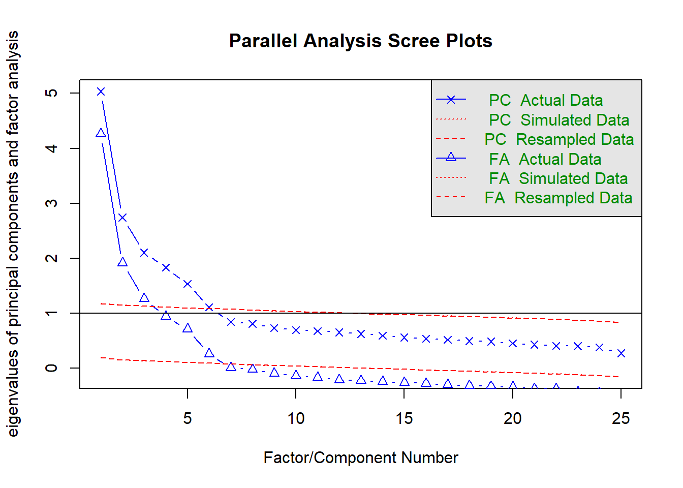
Third, we examine the scree and parallel analysis plot to help determine the number of factors. The scree-plot shows an elbow in the line that connects the eigenvalues of the factors at the seventh factor, which suggests that six factors should be retained. Parallel analysis also suggests that six factors should be extracted. This is somewhat surprising, given that the BFI is supposed to measure five personality factors.

fa.parallel(mydata)

Parallel analysis suggests that the number of factors =  6  and the number of components =  6 
#bfi.keys

#paSelect(bfi.keys, mydata, plot = TRUE)

Performing the EFA (round 1 with six factors)

Fourth, we perform the first exploratory factor analysis. We extract and rotate six factors. The factor loadings and factor correlations were estimated with the default “minres” (aka “unweighted least squares”) estimator. The factors were rotated to the default “direct oblimin” criterion.

Inspection of the rotated factor pattern matrix shows five well-defined factors that each have at least five salient factor loadings, and one poorly defined factor with three salient (but relatively low factor loadings that range from 0.30 to 0.41). The pattern of salient factor loadings (i.e. loadings > 0.30) indicate that the the first factor corresponds with Neuroticism, the second with Extroversion, the third with Conscientiousness, the fourth with Agreeableness, and the fifth with Openness. The psychological meaning of the sixth factor, which is loaded by one Conscientiousness item and two Openness items, is not clear.

my_efa <- fa(mydata, nfactors = 6)
print(my_efa, cut = .30)
Factor Analysis using method =  minres
Call: fa(r = mydata, nfactors = 6)
Standardized loadings (pattern matrix) based upon correlation matrix
     MR2   MR1   MR3   MR5   MR4   MR6   h2   u2 com
A1                   -0.56             0.34 0.66 1.7
A2                    0.68             0.50 0.50 1.1
A3                    0.61             0.51 0.49 1.2
A4                    0.39             0.28 0.72 2.1
A5                    0.45             0.47 0.53 2.3
C1              0.54                   0.34 0.66 1.3
C2              0.67                   0.49 0.51 1.3
C3              0.55                   0.31 0.69 1.1
C4             -0.64              0.30 0.57 0.43 1.5
C5             -0.54                   0.43 0.57 1.5
E1        0.59                         0.39 0.61 1.3
E2        0.70                         0.56 0.44 1.0
E3       -0.34              0.40       0.48 0.52 2.9
E4       -0.53                         0.55 0.45 1.9
E5       -0.40                         0.40 0.60 2.8
N1  0.84                               0.68 0.32 1.0
N2  0.83                               0.66 0.34 1.0
N3  0.67                               0.54 0.46 1.1
N4  0.43  0.42                         0.49 0.51 2.4
N5  0.44                               0.35 0.65 2.4
O1                          0.57       0.35 0.65 1.1
O2                         -0.36  0.36 0.29 0.71 2.4
O3                          0.65       0.48 0.52 1.1
O4        0.35              0.37       0.25 0.75 2.5
O5                         -0.45  0.41 0.37 0.63 2.0

                       MR2  MR1  MR3  MR5  MR4  MR6
SS loadings           2.48 2.17 2.05 1.88 1.68 0.82
Proportion Var        0.10 0.09 0.08 0.08 0.07 0.03
Cumulative Var        0.10 0.19 0.27 0.34 0.41 0.44
Proportion Explained  0.22 0.20 0.18 0.17 0.15 0.07
Cumulative Proportion 0.22 0.42 0.60 0.77 0.93 1.00

 With factor correlations of 
      MR2   MR1   MR3   MR5   MR4   MR6
MR2  1.00  0.25 -0.18 -0.10  0.02  0.16
MR1  0.25  1.00 -0.21 -0.30 -0.20 -0.08
MR3 -0.18 -0.21  1.00  0.19  0.19 -0.02
MR5 -0.10 -0.30  0.19  1.00  0.25  0.14
MR4  0.02 -0.20  0.19  0.25  1.00  0.02
MR6  0.16 -0.08 -0.02  0.14  0.02  1.00

Mean item complexity =  1.7
Test of the hypothesis that 6 factors are sufficient.

df null model =  300  with the objective function =  7.23 with Chi Square =  20163.79
df of  the model are 165  and the objective function was  0.37 

The root mean square of the residuals (RMSR) is  0.02 
The df corrected root mean square of the residuals is  0.03 

The harmonic n.obs is  2762 with the empirical chi square  639.91  with prob <  4.1e-57 
The total n.obs was  2800  with Likelihood Chi Square =  1032.48  with prob <  1.8e-125 

Tucker Lewis Index of factoring reliability =  0.92
RMSEA index =  0.043  and the 90 % confidence intervals are  0.041 0.046
BIC =  -277.19
Fit based upon off diagonal values = 0.99
Measures of factor score adequacy             
                                                   MR2  MR1  MR3  MR5  MR4  MR6
Correlation of (regression) scores with factors   0.93 0.89 0.89 0.87 0.86 0.77
Multiple R square of scores with factors          0.86 0.79 0.78 0.76 0.73 0.59
Minimum correlation of possible factor scores     0.72 0.59 0.57 0.53 0.46 0.17

Performing the EFA (round 2 with five factors)

my_efa2 <- fa(mydata, nfactors = 5)
print(my_efa2, cut = .30)
Factor Analysis using method =  minres
Call: fa(r = mydata, nfactors = 5)
Standardized loadings (pattern matrix) based upon correlation matrix
     MR2   MR1   MR3   MR5   MR4   h2   u2 com
A1                   -0.41       0.19 0.81 2.0
A2                    0.64       0.45 0.55 1.0
A3                    0.66       0.52 0.48 1.1
A4                    0.43       0.28 0.72 1.7
A5                    0.53       0.46 0.54 1.5
C1              0.55             0.33 0.67 1.2
C2              0.67             0.45 0.55 1.2
C3              0.57             0.32 0.68 1.1
C4             -0.61             0.45 0.55 1.2
C5             -0.55             0.43 0.57 1.4
E1       -0.56                   0.35 0.65 1.2
E2       -0.68                   0.54 0.46 1.1
E3        0.42                   0.44 0.56 2.6
E4        0.59                   0.53 0.47 1.5
E5        0.42                   0.40 0.60 2.6
N1  0.81                         0.65 0.35 1.1
N2  0.78                         0.60 0.40 1.0
N3  0.71                         0.55 0.45 1.1
N4  0.47 -0.39                   0.49 0.51 2.3
N5  0.49                         0.35 0.65 2.0
O1                          0.51 0.31 0.69 1.1
O2                         -0.46 0.26 0.74 1.7
O3                          0.61 0.46 0.54 1.2
O4       -0.32              0.37 0.25 0.75 2.7
O5                         -0.54 0.30 0.70 1.2

                       MR2  MR1  MR3  MR5  MR4
SS loadings           2.57 2.20 2.03 1.99 1.59
Proportion Var        0.10 0.09 0.08 0.08 0.06
Cumulative Var        0.10 0.19 0.27 0.35 0.41
Proportion Explained  0.25 0.21 0.20 0.19 0.15
Cumulative Proportion 0.25 0.46 0.66 0.85 1.00

 With factor correlations of 
      MR2   MR1   MR3   MR5   MR4
MR2  1.00 -0.21 -0.19 -0.04 -0.01
MR1 -0.21  1.00  0.23  0.33  0.17
MR3 -0.19  0.23  1.00  0.20  0.19
MR5 -0.04  0.33  0.20  1.00  0.19
MR4 -0.01  0.17  0.19  0.19  1.00

Mean item complexity =  1.5
Test of the hypothesis that 5 factors are sufficient.

df null model =  300  with the objective function =  7.23 with Chi Square =  20163.79
df of  the model are 185  and the objective function was  0.65 

The root mean square of the residuals (RMSR) is  0.03 
The df corrected root mean square of the residuals is  0.04 

The harmonic n.obs is  2762 with the empirical chi square  1392.16  with prob <  5.6e-184 
The total n.obs was  2800  with Likelihood Chi Square =  1808.94  with prob <  4.3e-264 

Tucker Lewis Index of factoring reliability =  0.867
RMSEA index =  0.056  and the 90 % confidence intervals are  0.054 0.058
BIC =  340.53
Fit based upon off diagonal values = 0.98
Measures of factor score adequacy             
                                                   MR2  MR1  MR3  MR5  MR4
Correlation of (regression) scores with factors   0.92 0.89 0.88 0.88 0.84
Multiple R square of scores with factors          0.85 0.79 0.77 0.77 0.71
Minimum correlation of possible factor scores     0.70 0.59 0.54 0.54 0.42

Comparing the fit of the 5-factor and 6-factor solutions

Fit_6factor <- c(my_efa$CFI, my_efa$TLI, my_efa$RMSEA, 
                 my_efa$rms, my_efa$fit.off, my_efa$BIC)

Fit_5factor <- c(my_efa2$CFI, my_efa2$TLI, my_efa2$RMSEA, 
                 my_efa2$rms, my_efa2$fit.off, my_efa2$BIC)

Fit_models <- cbind(Fit_5factor, Fit_6factor)

row.names(Fit_models) <- c("CFI", "TLI", "RMSEA", "  lower", "  upper",
                           "  confidence", "SRMR", "GFI", "BIC")

Fit_models
              Fit_5factor   Fit_6factor
CFI            0.91824607    0.95632879
TLI            0.86726507    0.92048207
RMSEA          0.05599015    0.04333042
  lower        0.05366671    0.04082710
  upper        0.05836612    0.04589177
  confidence   0.90000000    0.90000000
SRMR           0.02898448    0.01965083
GFI            0.98034412    0.99096510
BIC          340.52846609 -277.19122742

Evaluating the items with respect to their primary factor loadings

print(my_efa2, sort = TRUE, cut = .30)
Factor Analysis using method =  minres
Call: fa(r = mydata, nfactors = 5)
Standardized loadings (pattern matrix) based upon correlation matrix
   item   MR2   MR1   MR3   MR5   MR4   h2   u2 com
N1   16  0.81                         0.65 0.35 1.1
N2   17  0.78                         0.60 0.40 1.0
N3   18  0.71                         0.55 0.45 1.1
N5   20  0.49                         0.35 0.65 2.0
N4   19  0.47 -0.39                   0.49 0.51 2.3
E2   12       -0.68                   0.54 0.46 1.1
E4   14        0.59                   0.53 0.47 1.5
E1   11       -0.56                   0.35 0.65 1.2
E5   15        0.42                   0.40 0.60 2.6
E3   13        0.42                   0.44 0.56 2.6
C2    7              0.67             0.45 0.55 1.2
C4    9             -0.61             0.45 0.55 1.2
C3    8              0.57             0.32 0.68 1.1
C5   10             -0.55             0.43 0.57 1.4
C1    6              0.55             0.33 0.67 1.2
A3    3                    0.66       0.52 0.48 1.1
A2    2                    0.64       0.45 0.55 1.0
A5    5                    0.53       0.46 0.54 1.5
A4    4                    0.43       0.28 0.72 1.7
A1    1                   -0.41       0.19 0.81 2.0
O3   23                          0.61 0.46 0.54 1.2
O5   25                         -0.54 0.30 0.70 1.2
O1   21                          0.51 0.31 0.69 1.1
O2   22                         -0.46 0.26 0.74 1.7
O4   24       -0.32              0.37 0.25 0.75 2.7

                       MR2  MR1  MR3  MR5  MR4
SS loadings           2.57 2.20 2.03 1.99 1.59
Proportion Var        0.10 0.09 0.08 0.08 0.06
Cumulative Var        0.10 0.19 0.27 0.35 0.41
Proportion Explained  0.25 0.21 0.20 0.19 0.15
Cumulative Proportion 0.25 0.46 0.66 0.85 1.00

 With factor correlations of 
      MR2   MR1   MR3   MR5   MR4
MR2  1.00 -0.21 -0.19 -0.04 -0.01
MR1 -0.21  1.00  0.23  0.33  0.17
MR3 -0.19  0.23  1.00  0.20  0.19
MR5 -0.04  0.33  0.20  1.00  0.19
MR4 -0.01  0.17  0.19  0.19  1.00

Mean item complexity =  1.5
Test of the hypothesis that 5 factors are sufficient.

df null model =  300  with the objective function =  7.23 with Chi Square =  20163.79
df of  the model are 185  and the objective function was  0.65 

The root mean square of the residuals (RMSR) is  0.03 
The df corrected root mean square of the residuals is  0.04 

The harmonic n.obs is  2762 with the empirical chi square  1392.16  with prob <  5.6e-184 
The total n.obs was  2800  with Likelihood Chi Square =  1808.94  with prob <  4.3e-264 

Tucker Lewis Index of factoring reliability =  0.867
RMSEA index =  0.056  and the 90 % confidence intervals are  0.054 0.058
BIC =  340.53
Fit based upon off diagonal values = 0.98
Measures of factor score adequacy             
                                                   MR2  MR1  MR3  MR5  MR4
Correlation of (regression) scores with factors   0.92 0.89 0.88 0.88 0.84
Multiple R square of scores with factors          0.85 0.79 0.77 0.77 0.71
Minimum correlation of possible factor scores     0.70 0.59 0.54 0.54 0.42

Evaluating the items with respect to complexity

print(my_efa2, sort = TRUE)
Factor Analysis using method =  minres
Call: fa(r = mydata, nfactors = 5)
Standardized loadings (pattern matrix) based upon correlation matrix
   item   MR2   MR1   MR3   MR5   MR4   h2   u2 com
N1   16  0.81  0.10  0.00 -0.11 -0.05 0.65 0.35 1.1
N2   17  0.78  0.04  0.01 -0.09  0.01 0.60 0.40 1.0
N3   18  0.71 -0.10 -0.04  0.08  0.02 0.55 0.45 1.1
N5   20  0.49 -0.20  0.00  0.21 -0.15 0.35 0.65 2.0
N4   19  0.47 -0.39 -0.14  0.09  0.08 0.49 0.51 2.3
E2   12  0.10 -0.68 -0.02 -0.05 -0.06 0.54 0.46 1.1
E4   14  0.01  0.59  0.02  0.29 -0.08 0.53 0.47 1.5
E1   11 -0.06 -0.56  0.11 -0.08 -0.10 0.35 0.65 1.2
E5   15  0.15  0.42  0.27  0.05  0.21 0.40 0.60 2.6
E3   13  0.08  0.42  0.00  0.25  0.28 0.44 0.56 2.6
C2    7  0.15 -0.09  0.67  0.08  0.04 0.45 0.55 1.2
C4    9  0.17  0.00 -0.61  0.04 -0.05 0.45 0.55 1.2
C3    8  0.03 -0.06  0.57  0.09 -0.07 0.32 0.68 1.1
C5   10  0.19 -0.14 -0.55  0.02  0.09 0.43 0.57 1.4
C1    6  0.07 -0.03  0.55 -0.02  0.15 0.33 0.67 1.2
A3    3 -0.03  0.12  0.02  0.66  0.03 0.52 0.48 1.1
A2    2 -0.02  0.00  0.08  0.64  0.03 0.45 0.55 1.0
A5    5 -0.11  0.23  0.01  0.53  0.04 0.46 0.54 1.5
A4    4 -0.06  0.06  0.19  0.43 -0.15 0.28 0.72 1.7
A1    1  0.21  0.17  0.07 -0.41 -0.06 0.19 0.81 2.0
O3   23  0.03  0.15  0.02  0.08  0.61 0.46 0.54 1.2
O5   25  0.13  0.10 -0.03  0.04 -0.54 0.30 0.70 1.2
O1   21  0.02  0.10  0.07  0.02  0.51 0.31 0.69 1.1
O2   22  0.19  0.06 -0.08  0.16 -0.46 0.26 0.74 1.7
O4   24  0.13 -0.32 -0.02  0.17  0.37 0.25 0.75 2.7

                       MR2  MR1  MR3  MR5  MR4
SS loadings           2.57 2.20 2.03 1.99 1.59
Proportion Var        0.10 0.09 0.08 0.08 0.06
Cumulative Var        0.10 0.19 0.27 0.35 0.41
Proportion Explained  0.25 0.21 0.20 0.19 0.15
Cumulative Proportion 0.25 0.46 0.66 0.85 1.00

 With factor correlations of 
      MR2   MR1   MR3   MR5   MR4
MR2  1.00 -0.21 -0.19 -0.04 -0.01
MR1 -0.21  1.00  0.23  0.33  0.17
MR3 -0.19  0.23  1.00  0.20  0.19
MR5 -0.04  0.33  0.20  1.00  0.19
MR4 -0.01  0.17  0.19  0.19  1.00

Mean item complexity =  1.5
Test of the hypothesis that 5 factors are sufficient.

df null model =  300  with the objective function =  7.23 with Chi Square =  20163.79
df of  the model are 185  and the objective function was  0.65 

The root mean square of the residuals (RMSR) is  0.03 
The df corrected root mean square of the residuals is  0.04 

The harmonic n.obs is  2762 with the empirical chi square  1392.16  with prob <  5.6e-184 
The total n.obs was  2800  with Likelihood Chi Square =  1808.94  with prob <  4.3e-264 

Tucker Lewis Index of factoring reliability =  0.867
RMSEA index =  0.056  and the 90 % confidence intervals are  0.054 0.058
BIC =  340.53
Fit based upon off diagonal values = 0.98
Measures of factor score adequacy             
                                                   MR2  MR1  MR3  MR5  MR4
Correlation of (regression) scores with factors   0.92 0.89 0.88 0.88 0.84
Multiple R square of scores with factors          0.85 0.79 0.77 0.77 0.71
Minimum correlation of possible factor scores     0.70 0.59 0.54 0.54 0.42
fa_matrix <- data.frame(cbind(my_efa2$loadings, 
                   my_efa2$communality,
                   my_efa2$uniquenesses,
                   my_efa2$complexity))

fa_matrix <- fa_matrix %>%
  rename(communality = V6,
         uniqueness  = V7,
         complexity  = V8)

fa_matrix <- fa_matrix %>%
  mutate(across(where(is.numeric), round, 2))


fa_matrix %>% 
  arrange(complexity)
     MR2   MR1   MR3   MR5   MR4 communality uniqueness complexity
A2 -0.02  0.00  0.08  0.64  0.03        0.45       0.55       1.04
N2  0.78  0.04  0.01 -0.09  0.01        0.60       0.40       1.04
A3 -0.03  0.12  0.02  0.66  0.03        0.52       0.48       1.07
E2  0.10 -0.68 -0.02 -0.05 -0.06        0.54       0.46       1.07
N3  0.71 -0.10 -0.04  0.08  0.02        0.55       0.45       1.07
N1  0.81  0.10  0.00 -0.11 -0.05        0.65       0.35       1.08
C3  0.03 -0.06  0.57  0.09 -0.07        0.32       0.68       1.11
O1  0.02  0.10  0.07  0.02  0.51        0.31       0.69       1.13
C2  0.15 -0.09  0.67  0.08  0.04        0.45       0.55       1.17
O3  0.03  0.15  0.02  0.08  0.61        0.46       0.54       1.17
C4  0.17  0.00 -0.61  0.04 -0.05        0.45       0.55       1.18
C1  0.07 -0.03  0.55 -0.02  0.15        0.33       0.67       1.19
E1 -0.06 -0.56  0.11 -0.08 -0.10        0.35       0.65       1.21
O5  0.13  0.10 -0.03  0.04 -0.54        0.30       0.70       1.21
C5  0.19 -0.14 -0.55  0.02  0.09        0.43       0.57       1.44
A5 -0.11  0.23  0.01  0.53  0.04        0.46       0.54       1.49
E4  0.01  0.59  0.02  0.29 -0.08        0.53       0.47       1.49
A4 -0.06  0.06  0.19  0.43 -0.15        0.28       0.72       1.74
O2  0.19  0.06 -0.08  0.16 -0.46        0.26       0.74       1.75
N5  0.49 -0.20  0.00  0.21 -0.15        0.35       0.65       1.96
A1  0.21  0.17  0.07 -0.41 -0.06        0.19       0.81       1.97
N4  0.47 -0.39 -0.14  0.09  0.08        0.49       0.51       2.27
E3  0.08  0.42  0.00  0.25  0.28        0.44       0.56       2.55
E5  0.15  0.42  0.27  0.05  0.21        0.40       0.60       2.60
O4  0.13 -0.32 -0.02  0.17  0.37        0.25       0.75       2.69
## Plot the item complexities
labels <- names(my_efa2$complexity)

item.complexity <- data.frame(labels, my_efa2$complexity)
colnames(item.complexity) <- c("Item", "Complexity")

ggplot(item.complexity, 
       aes(x = reorder(Item, Complexity), 
           y = Complexity)) +
  geom_point() +
  labs(x = "Items", 
       y = "Complexity", 
       title = "Complexity of the BFI items") +
  theme(axis.text.x = element_text(angle = 90, 
                                   hjust = 1))

Examining the replicability of the factors

We can also examine the internal replicability of the five and six-factor solutions. Factors that do not replicate across different samples of persons from the same population are of less scientific interest than factors that do replicate across different samples.

Ideally, the replication process should be repeated several times. With each round the random samples will be different. If a consistent pattern emerges across the different rounds of analyses greater confidence can be placed in the results.

Randomly split the data into two data frames

ncases <- nrow(mydata)
prop1  <- 0.6
prop2  <- 1 - prop1 

tf <- as.vector(c(rep(TRUE,  prop1*ncases),
                  rep(FALSE, prop2*ncases))) 

tf.random <- sample(tf)   # Randomly shuffle TRUE and FALSE 

data1 <- mydata[tf.random,  ]   # Select the rows corresponding with TRUE
data2 <- mydata[!tf.random, ]   # Select the rows that don't correspond with TRUE (i.e. FALSE)

library(psych)
nrow(data1)
[1] 1680

Perform the factor analysis on sample 1

my_efa_s1 <- fa(data1, nfactors = 6)

Perform the factor analysis on sample 2

The factor pattern matrix of sample 2 is rotated to a target defined by the rotated factor pattern matrix of sample 1. This will ensure that the factors of sample 2 are as similar as possible to those of sample 1.

my_efa_s2  <- fa(data2, nfactors = 6)

my_efa_s2_t <- target.rot(my_efa_s2$loadings, my_efa_s1$loadings)

Examine the similarity of the factors in sample 1 and sample 2

fa.congruence(my_efa_s1, my_efa_s2_t)
      MR2   MR1   MR3   MR5   MR4   MR6
MR2  0.99  0.14 -0.01 -0.08 -0.01  0.09
MR1  0.14  0.99 -0.19 -0.07 -0.13 -0.13
MR5 -0.01 -0.19  0.99  0.10  0.10  0.13
MR3 -0.08 -0.07  0.10  0.98  0.10  0.05
MR4 -0.01 -0.13  0.10  0.10  0.99 -0.13
MR6  0.09 -0.12  0.13  0.05 -0.12  0.97