Introduction

At times an analyst may want to randomly split a sample into two. A common reason might be that the analyst wants to use the data of the first random sample to develop a model, and the data of the second random sample to test the model.

To demonstrate how this can be done I create a toy data frame with two variables, A and B, and ten cases.

A <- c(5, 7, 6, 8, 7, 9, 8, 10, 9, 11)
B <- c(12, 14, 16, 18, 20, 22, 24, 26, 28, 30)

df <- data.frame(A, B)
df

I want to split the data frame randomly into two, where the first data frame should contain 60% of the cases, and the second 40%. First, I specify the proportion of people that should be in the first random sample. Here I want 60% of the cases to be in random sample 1.

prop1 <- 0.6
prop2 <- 1 - prop1

Second, I create a vector, labeled tf, that contains in succession the desired proportions of TRUE (prop1) and FALSE (prop2). This vector contains as many entries as there are rows in the data frame.

tf    <- as.vector(c(rep(TRUE,  prop1*nrow(df)),
                     rep(FALSE, prop2*nrow(df))))

As an alternative, the exact number of persons that should be in the two samples can also be directly entered. Here we want six cases in the first sample and four in the second sample.

tf    <- as.vector(c(rep(TRUE,  6),
                     rep(FALSE, 4)))

Third, I specify seeds, which will allow the same random samples of TRUE and FALSE to be drawn if the analysis is repeated. If the seeds are not specified the random allocation will differ across different analyses. Fourth, the tf vector is randomly shuffled by drawing a random sample without replacement of equal length to the number of cases and store this as tf.random. This vector contains a random selection of TRUE and FALSE that corresponds with the specified proportions.

set.seed(12345)

tf.random   <- sample(tf)   # Randomly shuffle TRUE and FALSE

Fifth, the first random sample is drawn from the data frame, df (the entries corresponding with TRUE) and stored as data1. Sixth, the second random sample is drawn by excluding those in the first random sample and stored as data2.

When printed, it can be seen that the first random sample consists of six cases (60%), and the second of four cases (40%).

data1 <- df[tf.random,  ]   # Select the rows corresponding with TRUE
data2 <- df[!tf.random, ]   # Select the rows that don't correspond with TRUE (i.e. FALSE)

data1

data2

Putting the code together

To use this code users must (a) specifiy the proportion of cases that should be in the first data frame, and (b) replace df with the name of their data frame.

prop1 <- 0.6
prop2 <- 1 - prop1

tf    <- as.vector(c(rep(TRUE,  prop1*nrow(df)),
                     rep(FALSE, prop2*nrow(df)))) 

set.seed(12345)

tf.random   <- sample(tf)   # Randomly shuffle TRUE and FALSE 

data1 <- df[tf.random,  ]   # Select the rows corresponding with TRUE
data2 <- df[!tf.random, ]   # Select the rows that don't correspond with TRUE (i.e. FALSE)

data1

data2

Application with real data

The number of replicable factors in the Big Five Inventory

As an example I examine the replicability of the factors in the Big Five Inventory using exploratory factor analysis and the Burt-Tucker coefficient of congruence. The bfi data frame is included in the psychTools package. Each of the Big Five personality traits are measured by five items. The 25 personality items are in columns 1 to 25. Data are available for 2800 people. For ease of use I store the bfi data frame as df.

library(psychTools)
library(psych)
data(bfi)
df <- bfi

Parallel analysis and scree-plot

First, I examine the results of a parallel analysis and the scree-plot for the total sample, which suggest that six factors should be retained. This is counter to the theoretical expectation of five factors. The viability of a factor depends in part on whether it is replicable across different samples. A factor that does not replicate across different samples and different settings appear far less theoretically interesting and practically useful than a factor that replicates across samples and settings.

fa.parallel(df[1:25])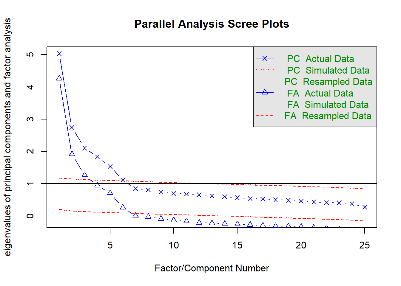

Parallel analysis suggests that the number of factors =  6  and the number of components =  6

Randomly split the data into two data frames

To examine the replicability of the factors I divide the data frame randomly in half.

prop1 <- 0.5
prop2 <- 1 - prop1

#tf    <- as.vector(c(rep(TRUE,  prop1*nrow(df)),
#                     rep(FALSE, prop2*nrow(df)))) 

tf <- as.vector(c(rep(TRUE,  1400),
                     rep(FALSE, 1400))) 

set.seed(12345)

tf.random <- sample(tf)   # Randomly shuffle TRUE and FALSE 

data1 <- df[tf.random,  ]   # Select the rows corresponding with TRUE
data2 <- df[!tf.random, ]   # Select the rows that don't correspond with TRUE (i.e. FALSE)

library(psych)
nrow(data1)

[1] 1400

nrow(data2)

[1] 1400

Factor analysis of the data of random sample 1

I perform the analysis with the first random sample, specifying six factors. By default the factors are extracted with unweighted least squares and rotated according to the Direct Quartimin (oblimin) criterion.

fa1 <- fa(data1[1:25], nfactors = 6)

Loading required namespace: GPArotation

Factor analysis of the data of random sample 2

I perform exactly the same analysis with the second random sample. I then use target rotation (aka Procrustes rotation) to maximise the similarity of the factors of sample 2 with those of sample 1.

fa2  <- fa(data2[1:25], nfactors = 6)

fa2t <- target.rot(fa2$loadings, fa1$loadings)

Similarity of the factors across the two samples

The replicability of the factors is examined by means of the Burt-Tucker coefficient of congruence. The coefficient of congruence for five of the six factors was 0.99, which indicates that these factors replicated very well across the two random samples. The coefficient of the sixth factor was 0.94, which is on the border of fair vs good factor similarity. This factor did not replicate as well as the other factors. Moreover, this factor was weakly defined in both samples and it does not appear to be psychologically meaningful. Jointly, these results raises questions about whether the sixth factor should be retained.

fa.congruence(fa1, fa2t)

      MR2   MR1   MR3   MR5   MR4   MR6
MR2  0.99  0.13 -0.05 -0.03 -0.01  0.12
MR1  0.13  0.99 -0.10 -0.17 -0.10 -0.17
MR3 -0.05 -0.10  0.99  0.09  0.08  0.02
MR5 -0.03 -0.17  0.09  0.99  0.05  0.14
MR4 -0.01 -0.10  0.08  0.05  0.99 -0.08
MR6  0.12 -0.16  0.01  0.13 -0.07  0.94

print(fa1$loadings, cut = 0)


Loadings:
   MR2    MR1    MR3    MR5    MR4    MR6   
A1  0.080 -0.105  0.030 -0.536 -0.007  0.279
A2  0.031 -0.036  0.048  0.694 -0.021 -0.058
A3 -0.023 -0.092  0.034  0.642  0.040  0.078
A4 -0.117 -0.041  0.187  0.360 -0.112  0.157
A5 -0.136 -0.197  0.002  0.447  0.105  0.201
C1  0.052  0.005  0.498 -0.084  0.150  0.076
C2  0.093  0.121  0.664  0.025  0.067  0.173
C3  0.048  0.031  0.536  0.092 -0.063  0.008
C4  0.067  0.036 -0.684 -0.050  0.016  0.224
C5  0.171  0.169 -0.542  0.007  0.045 -0.028
E1 -0.140  0.617  0.083 -0.105 -0.101  0.160
E2  0.070  0.695 -0.035 -0.060 -0.035 -0.009
E3 -0.006 -0.395 -0.029  0.146  0.337  0.244
E4 -0.034 -0.572  0.043  0.161 -0.056  0.254
E5  0.165 -0.432  0.242  0.044  0.178  0.010
N1  0.830 -0.109 -0.009 -0.073 -0.037 -0.024
N2  0.831 -0.052  0.008 -0.025 -0.020 -0.090
N3  0.683  0.138  0.000  0.035  0.053  0.144
N4  0.431  0.411 -0.130  0.049  0.078  0.085
N5  0.463  0.222 -0.016  0.148 -0.098  0.141
O1 -0.046 -0.066  0.056 -0.043  0.535  0.121
O2  0.110 -0.009 -0.123  0.155 -0.414  0.238
O3 -0.011 -0.117 -0.005  0.050  0.630  0.053
O4  0.142  0.315 -0.027  0.135  0.383  0.003
O5  0.067 -0.105 -0.051 -0.033 -0.506  0.285

                 MR2   MR1   MR3   MR5   MR4   MR6
SS loadings    2.427 2.020 1.886 1.671 1.496 0.601
Proportion Var 0.097 0.081 0.075 0.067 0.060 0.024
Cumulative Var 0.097 0.178 0.253 0.320 0.380 0.404

fa2t


Call: NULL
Standardized loadings (pattern matrix) based upon correlation matrix
     MR2   MR1   MR3   MR5   MR4   MR6   h2   u2
A1  0.13 -0.17  0.05 -0.56  0.00  0.32 0.46 0.54
A2  0.06 -0.01  0.13  0.68  0.04 -0.08 0.50 0.50
A3 -0.01 -0.16  0.02  0.59  0.05  0.14 0.39 0.61
A4 -0.02 -0.08  0.19  0.42 -0.14  0.13 0.25 0.75
A5 -0.17 -0.23 -0.01  0.46  0.06  0.25 0.35 0.65
C1  0.02  0.07  0.55 -0.04  0.19  0.15 0.40 0.60
C2  0.10  0.09  0.63  0.01  0.08  0.26 0.54 0.46
C3  0.01  0.06  0.56  0.07 -0.06  0.12 0.35 0.65
C4  0.07  0.08 -0.65 -0.04  0.00  0.32 0.50 0.50
C5  0.15  0.16 -0.57 -0.02  0.15  0.10 0.39 0.61
E1 -0.08  0.57  0.10 -0.13 -0.06  0.05 0.38 0.62
E2  0.07  0.68 -0.03 -0.06 -0.06  0.07 0.49 0.51
E3  0.03 -0.36 -0.01  0.16  0.34  0.26 0.34 0.66
E4 -0.06 -0.56 -0.02  0.24 -0.02  0.32 0.43 0.57
E5  0.14 -0.40  0.29  0.05  0.24  0.05 0.33 0.67
N1  0.83 -0.10  0.02 -0.09 -0.07  0.00 0.72 0.28
N2  0.83 -0.06  0.03 -0.07  0.01 -0.07 0.71 0.29
N3  0.67  0.11 -0.08  0.09  0.03  0.05 0.48 0.52
N4  0.45  0.41 -0.16  0.09  0.11  0.07 0.41 0.59
N5  0.43  0.22 -0.02  0.20 -0.15  0.17 0.32 0.68
O1 -0.02 -0.07  0.05 -0.06  0.57  0.11 0.36 0.64
O2  0.13 -0.04 -0.08  0.04 -0.43  0.36 0.30 0.70
O3  0.00 -0.14  0.02  0.00  0.65  0.09 0.46 0.54
O4  0.08  0.36 -0.04  0.15  0.39  0.04 0.31 0.69
O5  0.02 -0.03 -0.05 -0.02 -0.54  0.38 0.39 0.61

                       MR2  MR1  MR3  MR5  MR4  MR6
SS loadings           2.35 1.93 1.98 1.74 1.68 0.88
Proportion Var        0.09 0.08 0.08 0.07 0.07 0.04
Cumulative Var        0.09 0.17 0.25 0.32 0.39 0.42
Proportion Explained  0.22 0.18 0.19 0.16 0.16 0.08
Cumulative Proportion 0.22 0.41 0.59 0.76 0.92 1.00
      MR2   MR1   MR3   MR5   MR4   MR6
MR2  1.00 -0.03 -0.02  0.03 -0.02 -0.07
MR1 -0.03  1.00  0.03 -0.04  0.00  0.13
MR3 -0.02  0.03  1.00  0.00  0.03  0.11
MR5  0.03 -0.04  0.00  1.00  0.02 -0.04
MR4 -0.02  0.00  0.03  0.02  1.00  0.10
MR6 -0.07  0.13  0.11 -0.04  0.10  1.00