Department of Industrial Psychology, Stellenbosch University
Published
January 21, 2025
Introduction
In this tutorial I demonstrate how to calculate Cronbach’s coefficient alpha. The tutorial consists of four parts:
Calculating alpha from item covariances using R as a simple calculator
Calculating standardized alpha from item correlations using R as a simple calculator
Calculating alpha with the alpha() function of Bill Revelle’s psych package
Calculating confidence intervals via Feldt’s formula and bootstrapping
The calculation of alpha is demonstrated with the five Neuroticism items of the Big Five inventory, which is included in Revelle’s psychTools package in the bfi data set.
The assumptions underlying coefficient alpha
The calculation of coefficient alpha proceeds on the assumption that (a) the items constitute a unidimensional scale, and (b) the items are essentially tau-equivalent. The consequences of violating these assumptions are that the reliability coefficient may be biased. In practice, the assumption of essential tau-equivalence means that the unstandardized factor loadings of the items must be equal. This is rarely the case with real data, but if the factor loadings are “more or less equal”, the violation of the assumption does not have a major impact.
The violation of the assumption of unidimensionality is a different matter. Alpha, like all reliability coefficients, represents the ratio of true variance to total variance. Ideally, the true variance reflect the influence of single factor that represents the construct of interest. When there are multiple common factors, the reliability coefficient represents the ratio of the the true variance–that now reflects the influence of all the common factors–to the total variance. In such case it is not clear at all what the psychological meaning of the true variance is and the reliability coefficient also loses meaning. Best practice is to create unidimensional scales that have a clear psychological meaning and to then calculate the reliabilities of such unidimensional scales.
In cases where a scale measures a single dominant general factor and there are also some minor additional factors present, it may be best to estimate the reliability of the general factor with a coefficient called omega hierarchical.
Calculation of coefficient alpha of the Neuroticism Scale of the Big Five Inventory from the item variances and covariances
The total variance of a test is equal to sum of the item variances and twice the sum of the item covariances. The test variance can easily be obtained by simply summing all the elements of a square variance-covariance matrix of the items. Next, the ratio of the sum of the off-diagonal elements to the total variance is obtained. Finally, a correction for the number of items in the test is applied.
The variance-covariance matrix
First, we find the variance-covariance matrix of the test items. The variance-covariance matrix is a square matrix where the diagonal contains the item variances. The lower triangle of the matrix contains the covariances of pairs of items and this is mirrored in the upper triangle of the matrix.
library(psychTools)library(psych)data(bfi)mydata <- bfi[16:20]# Find the variance-covariance matrix of the itemsmycov <-cov(mydata, use ="complete.obs")mycov
The total test variance of a test, \(s^2\), is calculated by finding the sum of the elements of the covariance matrix, \(s^2 = \sum s^2_{i}+2\sum s^2_{ij}\). Here the test variance is \(35.70\).
In the R code below we find the sum of all the elements in the covariance matrix–which is labeled mycov and store it in an object we label A.
# Find the test variance by summing all the elements in the matrixA <-sum(mycov)A
[1] 35.69563
The sum of the item variances
Third, we calculate the sum of the item variances (i.e. the values on the diagonal of the matrix), \(\sum s^2_{i}\). The sum of the item variances is \(12.47\).
In R, we find the sum of the diagonal elements of mycov and store it as an object we label B.
# Find the sum of the item variancesB <-sum(diag(mycov))B
[1] 12.47053
The sum of the off diagonal elements
Next, we find the sum of the off-diagonal elements (i.e. \(2\sum s_{ij}\)). We only need to sum the values in the upper or lower triangle of the matrix and then multiply the sum by two.
In practice it is easier to find the sum of the off-diagonal elements by simply subtracting the sum of the item variances from the total test variance. Here the sum of the off-diagonal elements is \(35.70 - 12.47 = 23.23\).
In R, we find the sum of the item covariances \(\times\) 2 (all the off-diagonal elements in the covariance matrix) by subtracting the sum of the item variances (object B), from the total test variance (object A). We label the sum of the off-diagonal elements C.
# Subtract the item variances from the test variance to find the sum of the item covariancesC <- A - BC
[1] 23.22509
The ratio of the sum of the off-diagonal elements to the total test variance
Next, we find the ratio of the sum of the off-diagonal elements, \(2\sum s_{ij}\), to the total test variance, \(2\sum s_{ij} + \sum s_{i}^2\). Here \(23.23/35.70 = 0.65\).
In R, we divide the sum of the off-diagonal elements (object C) by the total test variance (object A).
# Obtain the ratio of the summed covariances to the test varianceC/A
[1] 0.6506425
Apply the correction for the number of items to obtain coefficient alpha
Finally, we apply the correction for the number of items in the test to obtain alpha.
We have to specify the number of items, k, which here is 5. Cronbach’s alpha coefficient of the 5-item Neuroticism scale is \(5/4 × 0.65 = 0.81\).
In R, we store the number of items as an object we label k. Next we multiple the ratio of the sum of the off-diagonal elements to the total test variance by k/(k-1).
# Specify the number of itemsk <-5# Apply the correction for the number of items to obtain coefficient alpha
k/(k-1)*C/A
[1] 0.8133031
Putting all the R code together
mycov <-cov(mydata, use ="complete.obs")A <-sum(mycov) ## The total test varianceB <-sum(diag(mycov)) ## Sum of diagonal elementsC <- A - B ## Sum of off-diagonal elements k <-5## Number of itemsk/(k-1)*C/A ## Coefficient alpha
[1] 0.8133031
Calculation of standardized coefficient alpha from the item correlation matrix
Standardized coefficient alpha can be obtained in the same way as unstandardized coefficient alpha by replacing the item variance-covariance matrix with the inter-item correlation matrix. When the data are standardized the item variances are all equal to unity and the sum of the item variances is equal to the number of items.
The item correlation matrix
First, we find the item correlation matrix. The item correlation matrix is also a square matrix. The diagonal contains the item variances, which are all equal to unity. The lower triangle of the matrix contains the correlations of pairs of items and this is mirrored in the upper triangle of the matrix.
Second, we calculate the test variance where all the items are standardized by summing across all the elements of the item correlation matrix. Here we store the total test variance as an object labeled D.
# Find the test variance by summing all the elements in the matrixD <-sum(cor(mydata, use ="complete.obs"))D
[1] 14.33723
The sum of the item variances
Third, we calculate the sum of the item variances (i.e. the values on the diagonal of the matrix). We store the sum of the item variances as an object labeled E. Note that the variance of a standardized item is equal to one. Therefore, the sum of the item variances is also simply equal to the number of items, k.
# Find the sum of the item variancesE <-sum(diag(cor(mydata, use ="complete.obs")))E
[1] 5
The sum of the off-diagonal elements
Next, we find the sum of the off-diagonal elements (i.e. \(2\times\sum(r_{ij})\)). We only need to sum the values in the upper or lower triangle of the matrix and then multiply the sum by two.
In practice it is easier to find the sum of the off-diagonal elements by simply subtracting the sum of the item variances from the total test variance. We store \(2\times\sum(r_{ij})\) as an object labeled F.
# Subtract the item variances from the test variance to find the sum of the item covariancesF <- D - EF
[1] 9.337232
The ratio of the sum of the off-diagonal elements to the total test variance
# Obtain the ratio of the summed covariances to the test varianceF/D
[1] 0.6512577
Apply the correction for the number of items to obtain coefficient alpha
Next, we apply the correction for the number of items in the test to obtain alpha. Note that the sum of the item variances in the numerator of the second term of the equation is replaced by k (because the sum of the variances of standardized items is equal to the number of items).
# Specify the number of itemsk <-5# Apply the correction for the number of items to obtain coefficient alpha
(k)/(k-1)*F/D
[1] 0.8140721
Finding coefficient alpha with the alpha() function of the psych package
In practice coefficient alpha can be obtained with the alpha() function of the psych package. This function yields unstandardized and standardized alpha in addition to detailed information about the functioning of the items. In this chapter the focus falls on the reliability coefficients. The chapter on item analysis will examine more closely the information about the functioning of the items.
First, we find the unstandardized (raw) and standardized alpha coefficients.
library(psych)alpha(mydata)$total[c(1,2)]
 raw_alpha std.alpha
 0.8139629 0.8145354
Finding the 95% confidence interval of coefficient alpha (Feldt’s formula)
The observed coefficient alpha is calculated with sample data. Feldt developed a formula that can be used to calculate a confidence interval of coefficient alpha. The alpha() function yields Feldt’s 95% confidence intervals which provides a range of plausible values for the population value of alpha.
Finding a bootstrapped 95% confidence interval of coefficient alpha
The 95% confidence interval can also be obtained empirically via bootstrapping. This entails repeatedly drawing m random samples with replacement from the observed data set. Each of the random samples with replacement contains the same number of observations (rows) as the observed data set. Within each of the m samples coefficient alpha is calculated. The standard deviation of the m coefficient alphas is used as an estimator of the standard error of alpha. In turn, the estimated standard error is used to construct the 95% confidence interval. The lower boundary is equal to the mean of the m alphas minus two times the standard error. The upper boundary is equal to the the mean of the m alphas plus two times the standard error.
Confidence intervals (Feldt or bootstrapped) are useful because they provide a range of plausible values for the population value of alpha.
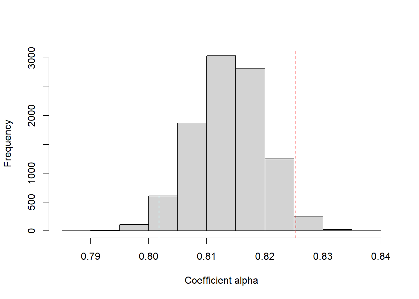
Users can specify how many random samples with replacement they want to draw from the observed data. Here the value is set at 10000 iterations (at each iteration a new random sample with replacement is drawn from the sample data). The results give a range of plausible values within which the population value of alpha lies (0.802 to 0.825). Note that because random samples are drawn, the values of the confidence intervals will change slightly each time the function is run.
Figure 4.1 is a histogram of coefficient alpha across the 10000 bootstrapped samples. The dashed lines represent the upper and lower boundaries of the 95% confidence intervals.
hist(alpha.boot$boot[,1], xlab ="Coefficient alpha", main =NULL)abline(v = alpha.boot$boot.ci[1], col ="red", lty ="dashed")abline(v = alpha.boot$boot.ci[3], col ="red", lty ="dashed")
Distribution of coefficient alpha across 10000 bootstrapped samples
Finding coefficient beta
Coefficient beta is the worst possible split-half reliability of the test. Beta is obtained by performing an item cluster analysis. Coefficient alpha and beta is calculated for each cluster. Coefficient beta is an indicator of the general factor saturation of a test, i.e. the proportion of the total test variance that is accounted for by a general factor. By contrast, coefficient alpha is an indicator of the proportion of total test variance that is accounted for by ALL sources of common variance among the items.
In a perfectly unidimensional test the lowest possible split-half, coefficient beta, will be equal to coefficient alpha, because there is only one source of common variance (i.e. the general factor). In practice, tests are never perfectly undimensional and beta will be lower than alpha. From this perspective the goal of an analysis is to determine if a scale has a general factor that is strong enough to justify the treatment of the scale as unidimensional. In this respect the discrepancy between alpha and beta is informative–the smaller the discrepancy the stronger the claim that the scale can be treated as unidimensional.
Figure 5.1 presents the results of an item cluster analysis of the Neuroticism Scale. All the items and sub-clusters converged into a single cluster with \(\alpha\) = 0.81 and \(\beta\) = 0.76. This suggests that the general factor underlying the nine items accounts for about 76% of the observed test variance.
beta <- psych::iclust(mydata, title =NULL)
Item cluster analysis of the items
beta$beta
       C4
0.7616692
Factors that influence coefficient alpha
The number of items and the strength of the inter-item covariances/correlations influence the size of coefficient alpha. Tests that contain more items will be more reliable that shorter tests, on condition that the items of the longer test are of the same quality than those of the shorter test. A point is reached after which the inclusion of additional items have a negligible effect on the test reliability.
A test with stronger inter-item covariances/correlations will be more reliable than a test of the same length with weaker inter-item covariances/correlations. This implies that we could obtain a very reliable test by repeatedly asking the same question, because the inter-item correlations will be very strong. Such a test would be of relatively little value, however. In practice, test developers strive to include items that all have a single latent attribute in common, yet each item must target a somewhat different aspect of the latent attribute. In this sense, all the items in a test must be the same, yet all the items must be different too!
Including items that are mere paraphrases of each other will inflate the reliability of the test, but at the cost of breadth of coverage. In turn, the narrowed breadth of coverage could constrain the validity of the test. This is known as the attenuation paradox. Test developers should take care not to include items that are mere paraphrases of each other in the test.
The strength of the inter-item correlations depends on the variance of the latent attribute in the sample from which the correlations are obtained. Restriction of range leads to weaker correlations.