Examining factor similarity across groups

R
psych
exploratory factor analysis
Author
Affiliation

Deon de Bruin

Department of Industrial Psychology, Stellenbosch University

Published

January 21, 2025

Introduction

In this tutorial I demonstrate how to examine the similarity of factor solutions across different groups with Tucker’s phi coefficient (aka Burt’s coefficient of congruence). Here I examine the similarity of the big five personality factors (as measured by the Big Five Inventory) of men and women with the fa(), fa.congruence(), and target.rot() functions of the psych package (Revelle, 2024a) in R. I use the bfi data set that is included in the psychtools (Revelle, 2024b) package. This data set contains the responses of 2800 people to the items of the Big Five Inventory. There are 919 men (coded as 1) and 1881 women (coded as 2).

Lorenzo-Seva and ten Berge’s (2006) excellent article describes the meaning of the coefficient of congruence and how it can be used to evaluate the similarity of factors across groups. They suggested that coefficients of congruence in the range 0.85 to 0.94 suggest fair similarity, while values above 0.95 suggest good similarity.

Descriptive statistics of the Big Five Inventory items

library(psychTools)
library(psych)
data(bfi)
mydata <- bfi
describe(mydata)
          vars    n  mean    sd median trimmed   mad min max range  skew
A1           1 2784  2.41  1.41      2    2.23  1.48   1   6     5  0.83
A2           2 2773  4.80  1.17      5    4.98  1.48   1   6     5 -1.12
A3           3 2774  4.60  1.30      5    4.79  1.48   1   6     5 -1.00
A4           4 2781  4.70  1.48      5    4.93  1.48   1   6     5 -1.03
A5           5 2784  4.56  1.26      5    4.71  1.48   1   6     5 -0.85
C1           6 2779  4.50  1.24      5    4.64  1.48   1   6     5 -0.85
C2           7 2776  4.37  1.32      5    4.50  1.48   1   6     5 -0.74
C3           8 2780  4.30  1.29      5    4.42  1.48   1   6     5 -0.69
C4           9 2774  2.55  1.38      2    2.41  1.48   1   6     5  0.60
C5          10 2784  3.30  1.63      3    3.25  1.48   1   6     5  0.07
E1          11 2777  2.97  1.63      3    2.86  1.48   1   6     5  0.37
E2          12 2784  3.14  1.61      3    3.06  1.48   1   6     5  0.22
E3          13 2775  4.00  1.35      4    4.07  1.48   1   6     5 -0.47
E4          14 2791  4.42  1.46      5    4.59  1.48   1   6     5 -0.82
E5          15 2779  4.42  1.33      5    4.56  1.48   1   6     5 -0.78
N1          16 2778  2.93  1.57      3    2.82  1.48   1   6     5  0.37
N2          17 2779  3.51  1.53      4    3.51  1.48   1   6     5 -0.08
N3          18 2789  3.22  1.60      3    3.16  1.48   1   6     5  0.15
N4          19 2764  3.19  1.57      3    3.12  1.48   1   6     5  0.20
N5          20 2771  2.97  1.62      3    2.85  1.48   1   6     5  0.37
O1          21 2778  4.82  1.13      5    4.96  1.48   1   6     5 -0.90
O2          22 2800  2.71  1.57      2    2.56  1.48   1   6     5  0.59
O3          23 2772  4.44  1.22      5    4.56  1.48   1   6     5 -0.77
O4          24 2786  4.89  1.22      5    5.10  1.48   1   6     5 -1.22
O5          25 2780  2.49  1.33      2    2.34  1.48   1   6     5  0.74
gender      26 2800  1.67  0.47      2    1.71  0.00   1   2     1 -0.73
education   27 2577  3.19  1.11      3    3.22  1.48   1   5     4 -0.05
age         28 2800 28.78 11.13     26   27.43 10.38   3  86    83  1.02
          kurtosis   se
A1           -0.31 0.03
A2            1.05 0.02
A3            0.44 0.02
A4            0.04 0.03
A5            0.16 0.02
C1            0.30 0.02
C2           -0.14 0.03
C3           -0.13 0.02
C4           -0.62 0.03
C5           -1.22 0.03
E1           -1.09 0.03
E2           -1.15 0.03
E3           -0.47 0.03
E4           -0.30 0.03
E5           -0.09 0.03
N1           -1.01 0.03
N2           -1.05 0.03
N3           -1.18 0.03
N4           -1.09 0.03
N5           -1.06 0.03
O1            0.43 0.02
O2           -0.81 0.03
O3            0.30 0.02
O4            1.08 0.02
O5           -0.24 0.03
gender       -1.47 0.01
education    -0.32 0.02
age           0.56 0.21

Choose the columns that contain the items

items <- c(1:25)   ### Type here the range of columns that contain the items
items
 [1]  1  2  3  4  5  6  7  8  9 10 11 12 13 14 15 16 17 18 19 20 21 22 23 24 25
test.length <- length(items)
test.length
[1] 25

Select the persons that represent the reference and focal groups

Here we choose the men (coded as 1) as the reference group and the women (coded as 2) as the focal group. We store the data of the reference group as personsR and those of the focal group as personsF.

personsR <- mydata[mydata$gender == 1, ] 
personsF <- mydata[mydata$gender == 2, ]

Specify the number of factors to retain

nfactors = 5

Specify the factor rotation criterion

The most popular oblique rotation criteria are direct oblimin, promax and geomin. The most popular orthogonal rotation criterion is variamax.

rotation <- c("oblimin")  ### Choose one of "oblimin", "promax", "geomin", or for an orthogonal solution "varimax"

Factor analysis results: reference group

Number of persons in the analysis: reference group

nrow(personsR)
[1] 919

Descriptive statistics of the item pool: reference group

          vars   n  mean    sd median trimmed  mad min max range  skew kurtosis
A1           1 918  2.73  1.43      2    2.62 1.48   1   6     5  0.56    -0.69
A2           2 908  4.50  1.26      5    4.65 1.48   1   6     5 -0.89     0.34
A3           3 912  4.34  1.33      5    4.47 1.48   1   6     5 -0.75    -0.11
A4           4 916  4.43  1.48      5    4.60 1.48   1   6     5 -0.76    -0.39
A5           5 915  4.38  1.32      5    4.51 1.48   1   6     5 -0.72    -0.20
C1           6 913  4.48  1.24      5    4.61 1.48   1   6     5 -0.80     0.17
C2           7 913  4.24  1.34      5    4.34 1.48   1   6     5 -0.61    -0.42
C3           8 910  4.20  1.32      4    4.30 1.48   1   6     5 -0.63    -0.35
C4           9 911  2.72  1.41      2    2.61 1.48   1   6     5  0.41    -0.86
C5          10 914  3.51  1.65      4    3.52 1.48   1   6     5 -0.13    -1.23
E1          11 913  3.27  1.66      3    3.21 1.48   1   6     5  0.15    -1.24
E2          12 913  3.27  1.61      3    3.21 1.48   1   6     5  0.12    -1.18
E3          13 908  3.91  1.40      4    3.97 1.48   1   6     5 -0.41    -0.63
E4          14 915  4.27  1.50      5    4.41 1.48   1   6     5 -0.70    -0.58
E5          15 915  4.29  1.37      5    4.40 1.48   1   6     5 -0.64    -0.36
N1          16 910  2.83  1.56      3    2.73 1.48   1   6     5  0.40    -1.04
N2          17 915  3.30  1.52      3    3.27 1.48   1   6     5  0.04    -1.07
N3          18 917  2.94  1.54      3    2.86 1.48   1   6     5  0.31    -1.08
N4          19 910  3.19  1.59      3    3.13 1.48   1   6     5  0.15    -1.14
N5          20 909  2.48  1.49      2    2.30 1.48   1   6     5  0.76    -0.54
O1          21 913  4.98  1.08      5    5.15 1.48   1   6     5 -1.15     1.22
O2          22 919  2.65  1.56      2    2.48 1.48   1   6     5  0.66    -0.70
O3          23 915  4.50  1.22      5    4.63 1.48   1   6     5 -0.87     0.56
O4          24 913  4.90  1.24      5    5.11 1.48   1   6     5 -1.21     0.97
O5          25 915  2.45  1.37      2    2.27 1.48   1   6     5  0.83    -0.14
gender      26 919  1.00  0.00      1    1.00 0.00   1   1     0   NaN      NaN
education   27 838  3.18  1.19      3    3.22 1.48   1   5     4 -0.10    -0.62
age         28 919 28.02 11.03     25   26.49 8.90   3  74    71  1.23     1.22
            se
A1        0.05
A2        0.04
A3        0.04
A4        0.05
A5        0.04
C1        0.04
C2        0.04
C3        0.04
C4        0.05
C5        0.05
E1        0.06
E2        0.05
E3        0.05
E4        0.05
E5        0.05
N1        0.05
N2        0.05
N3        0.05
N4        0.05
N5        0.05
O1        0.04
O2        0.05
O3        0.04
O4        0.04
O5        0.05
gender    0.00
education 0.04
age       0.36

Multidimensional factor solution: reference group

By default the factors were extracted using unweighted least squares (aka minimum residual or minres) and obliquely rotated according to the direct oblimin criterion. Inspection of the rotated factor pattern matrix shows that the first factor, labeled MR1, has high loadings on the Extroversion items (items E1 to E5), the second factor, labeled MR2, has high loadings on the Neuroticism items (items N1 to N5), the third factor, labeled MR5, has high loadings on four Agreeableness items (items A2 to A5 – the loading of item A1 “unexpectedly” was relatively low), the fourth factor, labeled MR3, has high loadings on the Conscientiousness items (items C1 to C5), and the fifth factor, labeled MR4, has high loadings on the Openness items (items O1 to O5). It appears safe to label the five factors of the reference group (the men) as Extroversion (MR1), Neuroticism (MR2), Agreeableness (MR5), Conscientiousness (MR3), and Openness (MR4).

library(psych)
options(digits = 3)
myfactorsR <- fa(personsR[, items], nfactors = nfactors, rotate = rotation)
Loading required namespace: GPArotation
myfactorsR
Factor Analysis using method =  minres
Call: fa(r = personsR[, items], nfactors = nfactors, rotate = rotation)
Standardized loadings (pattern matrix) based upon correlation matrix
     MR1   MR2   MR5   MR3   MR4   h2   u2 com
A1 -0.03  0.19 -0.26  0.08 -0.10 0.11 0.89 2.4
A2 -0.02 -0.05  0.59  0.08  0.04 0.39 0.61 1.1
A3 -0.06 -0.05  0.71 -0.01  0.06 0.55 0.45 1.0
A4 -0.03 -0.07  0.43  0.26 -0.09 0.30 0.70 1.8
A5 -0.19 -0.13  0.61  0.04  0.00 0.51 0.49 1.3
C1  0.08  0.06  0.06  0.57  0.15 0.37 0.63 1.2
C2  0.19  0.06  0.14  0.67  0.09 0.48 0.52 1.3
C3  0.01  0.05  0.09  0.57 -0.12 0.32 0.68 1.2
C4  0.14  0.14  0.17 -0.57 -0.09 0.45 0.55 1.5
C5  0.26  0.17  0.11 -0.53  0.07 0.47 0.53 1.8
E1  0.64 -0.04 -0.09  0.18 -0.15 0.44 0.56 1.3
E2  0.72  0.03 -0.09 -0.07 -0.02 0.61 0.39 1.1
E3 -0.36  0.05  0.34  0.01  0.27 0.44 0.56 2.9
E4 -0.53  0.00  0.40  0.03 -0.09 0.56 0.44 1.9
E5 -0.45  0.16  0.17  0.29  0.13 0.46 0.54 2.6
N1 -0.12  0.83 -0.11  0.05 -0.07 0.66 0.34 1.1
N2 -0.07  0.78 -0.10 -0.01  0.03 0.59 0.41 1.1
N3  0.16  0.65  0.12 -0.06  0.02 0.52 0.48 1.2
N4  0.38  0.46  0.09 -0.14  0.12 0.49 0.51 2.4
N5  0.27  0.39  0.15 -0.03 -0.11 0.29 0.71 2.3
O1 -0.02  0.02  0.09  0.07  0.53 0.33 0.67 1.1
O2  0.07  0.13  0.28 -0.06 -0.46 0.28 0.72 1.9
O3 -0.08  0.02  0.15  0.04  0.60 0.45 0.55 1.2
O4  0.34  0.07  0.16 -0.04  0.38 0.27 0.73 2.5
O5  0.03  0.12  0.19 -0.06 -0.56 0.35 0.65 1.4

                       MR1  MR2  MR5  MR3  MR4
SS loadings           2.35 2.35 2.27 2.10 1.61
Proportion Var        0.09 0.09 0.09 0.08 0.06
Cumulative Var        0.09 0.19 0.28 0.36 0.43
Proportion Explained  0.22 0.22 0.21 0.20 0.15
Cumulative Proportion 0.22 0.44 0.65 0.85 1.00

 With factor correlations of 
      MR1   MR2   MR5   MR3   MR4
MR1  1.00  0.22 -0.28 -0.25 -0.10
MR2  0.22  1.00  0.01 -0.20 -0.03
MR5 -0.28  0.01  1.00  0.15  0.18
MR3 -0.25 -0.20  0.15  1.00  0.18
MR4 -0.10 -0.03  0.18  0.18  1.00

Mean item complexity =  1.6
Test of the hypothesis that 5 factors are sufficient.

df null model =  300  with the objective function =  7.69 with Chi Square =  6986
df of  the model are 185  and the objective function was  0.77 

The root mean square of the residuals (RMSR) is  0.03 
The df corrected root mean square of the residuals is  0.04 

The harmonic n.obs is  908 with the empirical chi square  515  with prob <  6.2e-33 
The total n.obs was  919  with Likelihood Chi Square =  699  with prob <  9.2e-61 

Tucker Lewis Index of factoring reliability =  0.875
RMSEA index =  0.055  and the 90 % confidence intervals are  0.051 0.059
BIC =  -563
Fit based upon off diagonal values = 0.98
Measures of factor score adequacy             
                                                   MR1  MR2  MR5  MR3  MR4
Correlation of (regression) scores with factors   0.90 0.92 0.89 0.88 0.84
Multiple R square of scores with factors          0.81 0.84 0.80 0.78 0.71
Minimum correlation of possible factor scores     0.63 0.68 0.60 0.56 0.43

Factor analysis results: focal group

Number of persons in the analysis: focal group

[1] 1881

Descriptive statistics of the item pool: focal group

   vars    n mean   sd median trimmed  mad min max range  skew kurtosis   se
A1    1 1866 2.26 1.37      2    2.05 1.48   1   6     5  0.99     0.04 0.03
A2    2 1865 4.95 1.09      5    5.12 1.48   1   6     5 -1.24     1.55 0.03
A3    3 1862 4.73 1.27      5    4.93 1.48   1   6     5 -1.15     0.90 0.03
A4    4 1865 4.83 1.46      5    5.09 1.48   1   6     5 -1.20     0.41 0.03
A5    5 1869 4.65 1.22      5    4.80 1.48   1   6     5 -0.90     0.36 0.03
C1    6 1866 4.52 1.24      5    4.66 1.48   1   6     5 -0.88     0.37 0.03
C2    7 1863 4.43 1.30      5    4.58 1.48   1   6     5 -0.81     0.04 0.03
C3    8 1870 4.35 1.27      5    4.48 1.48   1   6     5 -0.72    -0.02 0.03
C4    9 1863 2.47 1.35      2    2.32 1.48   1   6     5  0.69    -0.46 0.03
C5   10 1870 3.19 1.61      3    3.12 1.48   1   6     5  0.16    -1.16 0.04
E1   11 1864 2.83 1.60      2    2.70 1.48   1   6     5  0.49    -0.96 0.04
E2   12 1871 3.08 1.60      3    2.99 1.48   1   6     5  0.27    -1.13 0.04
E3   13 1867 4.04 1.33      4    4.11 1.48   1   6     5 -0.49    -0.38 0.03
E4   14 1876 4.50 1.43      5    4.68 1.48   1   6     5 -0.88    -0.15 0.03
E5   15 1864 4.48 1.31      5    4.64 1.48   1   6     5 -0.85     0.07 0.03
N1   16 1868 2.98 1.57      3    2.87 1.48   1   6     5  0.36    -1.00 0.04
N2   17 1864 3.61 1.52      4    3.64 1.48   1   6     5 -0.14    -1.03 0.04
N3   18 1872 3.35 1.62      3    3.32 1.48   1   6     5  0.06    -1.20 0.04
N4   19 1854 3.18 1.56      3    3.12 1.48   1   6     5  0.22    -1.07 0.04
N5   20 1862 3.21 1.63      3    3.13 1.48   1   6     5  0.20    -1.15 0.04
O1   21 1865 4.73 1.14      5    4.87 1.48   1   6     5 -0.79     0.17 0.03
O2   22 1881 2.74 1.57      2    2.60 1.48   1   6     5  0.55    -0.87 0.04
O3   23 1857 4.41 1.22      5    4.52 1.48   1   6     5 -0.73     0.18 0.03
O4   24 1873 4.89 1.21      5    5.09 1.48   1   6     5 -1.22     1.13 0.03
O5   25 1865 2.51 1.31      2    2.37 1.48   1   6     5  0.69    -0.29 0.03

Multidimensional factor solution: focal group

Inspection of the rotated factor pattern matrix of the focal group shows that the first factor, labeled MR2, has high loadings on the Neuroticism items (items N1 to N5), the second factor, labeled MR1, has high loadings on the Extroversion items (items E1 to E5), the third factor, labeled MR3, has high loadings on the Conscientiousness items (items C1 to C5), the fourth factor, labeled MR5, has high loadings on the Agreeableness items (items A1 to A5), and the fifth factor, labeled MR4, has high loadings on the Openness items (items O1 to O5). It appears safe to label the five factors of the focal group (the women) as Neuroticism (MR2), Extroversion (MR1), Conscientiousness (MR3), Agreeableness (MR5), and Openness (MR4).

Whereas the order of the factors are different across the two groups, each of the big five factors were found for both the reference and the focal group. What remains to be seen is how similar the patterns of high and low loadings are across the two groups.

library(psych)
options(digits = 3)
myfactorsF <- fa(personsF[, items], nfactors = nfactors, rotate = rotation)
myfactorsF
Factor Analysis using method =  minres
Call: fa(r = personsF[, items], nfactors = nfactors, rotate = rotation)
Standardized loadings (pattern matrix) based upon correlation matrix
     MR2   MR1   MR3   MR5   MR4   h2   u2 com
A1  0.22  0.22  0.10 -0.44 -0.09 0.24 0.76 2.3
A2 -0.01  0.00  0.07  0.63  0.05 0.43 0.57 1.0
A3 -0.02  0.15  0.05  0.62  0.01 0.50 0.50 1.1
A4 -0.06  0.08  0.16  0.42 -0.18 0.26 0.74 1.8
A5 -0.10  0.26  0.00  0.48  0.05 0.43 0.57 1.7
C1  0.06  0.01  0.54 -0.06  0.13 0.32 0.68 1.2
C2  0.17 -0.02  0.68  0.05  0.00 0.46 0.54 1.1
C3  0.01 -0.09  0.56  0.10 -0.04 0.32 0.68 1.1
C4  0.21  0.06 -0.61  0.01 -0.06 0.46 0.54 1.3
C5  0.23 -0.08 -0.54 -0.02  0.08 0.41 0.59 1.5
E1 -0.04 -0.53  0.10 -0.06 -0.10 0.31 0.69 1.2
E2  0.16 -0.65  0.02 -0.04 -0.07 0.52 0.48 1.2
E3  0.10  0.45  0.01  0.23  0.25 0.44 0.56 2.2
E4 -0.01  0.61  0.03  0.25 -0.10 0.52 0.48 1.4
E5  0.12  0.39  0.27  0.01  0.24 0.37 0.63 2.7
N1  0.80  0.09 -0.01 -0.09 -0.04 0.65 0.35 1.1
N2  0.77  0.03  0.02 -0.10  0.02 0.60 0.40 1.0
N3  0.73 -0.06 -0.02  0.03  0.03 0.55 0.45 1.0
N4  0.51 -0.37 -0.12  0.09  0.06 0.49 0.51 2.1
N5  0.53 -0.16 -0.01  0.17 -0.15 0.36 0.64 1.6
O1  0.05  0.17  0.11  0.03  0.46 0.31 0.69 1.4
O2  0.21  0.09 -0.07  0.11 -0.48 0.28 0.72 1.6
O3  0.06  0.22  0.03  0.08  0.58 0.46 0.54 1.3
O4  0.19 -0.28  0.00  0.18  0.35 0.24 0.76 3.1
O5  0.10  0.11  0.01 -0.02 -0.56 0.31 0.69 1.2

                       MR2  MR1  MR3  MR5  MR4
SS loadings           2.73 2.17 1.99 1.80 1.55
Proportion Var        0.11 0.09 0.08 0.07 0.06
Cumulative Var        0.11 0.20 0.28 0.35 0.41
Proportion Explained  0.27 0.21 0.19 0.18 0.15
Cumulative Proportion 0.27 0.48 0.67 0.85 1.00

 With factor correlations of 
      MR2   MR1   MR3   MR5   MR4
MR2  1.00 -0.19 -0.17 -0.11 -0.02
MR1 -0.19  1.00  0.20  0.32  0.18
MR3 -0.17  0.20  1.00  0.20  0.19
MR5 -0.11  0.32  0.20  1.00  0.19
MR4 -0.02  0.18  0.19  0.19  1.00

Mean item complexity =  1.5
Test of the hypothesis that 5 factors are sufficient.

df null model =  300  with the objective function =  7.12 with Chi Square =  13313
df of  the model are 185  and the objective function was  0.68 

The root mean square of the residuals (RMSR) is  0.03 
The df corrected root mean square of the residuals is  0.04 

The harmonic n.obs is  1854 with the empirical chi square  931  with prob <  8.5e-100 
The total n.obs was  1881  with Likelihood Chi Square =  1262  with prob <  1.6e-159 

Tucker Lewis Index of factoring reliability =  0.866
RMSEA index =  0.056  and the 90 % confidence intervals are  0.053 0.059
BIC =  -133
Fit based upon off diagonal values = 0.98
Measures of factor score adequacy             
                                                   MR2  MR1  MR3  MR5  MR4
Correlation of (regression) scores with factors   0.93 0.89 0.87 0.86 0.84
Multiple R square of scores with factors          0.86 0.78 0.77 0.74 0.70
Minimum correlation of possible factor scores     0.71 0.57 0.53 0.49 0.40

Factor congruence coefficients

The rows of the table below represent the factors of the reference and the columns the factors of the focal group. The same number of factors were extracted in both groups and the same oblique rotation criterion was applied (by default direct oblimin).

Working our way across the rows of the matrix we see that factor MR1 (Extroversion) of the men has a coefficient of congruence of -0.92 with factor MR1 (Extroversion) of the women. The negative sign indicates that the poles of the factor of the men are opposite of that of the women. The direction of the poles is arbitrary and one could simply change the signs of all the factor loadings of factor MR1 of the women, which would yield a positive coefficient of congruence of 0.92. The remaining coefficients in the first row are all relatively small, which simply indicates that the Extroversion factor of the men is very dissimilar to the Neuroticism, Agreeableness, Consicientiousness, and Openness factors of the women. This is a good sign.

The second row shows that factor M2 of the men (Neuroticism) and factor M2 of the women (Neuroticism) has a coefficient of congruence of 0.98. This signifies that the pattern of high and low loadings on this factor is very similar across the two groups.

The third row shows that factor M5 of the men (Agreeableness) and factor M5 of the women (Agreeableness) has a coefficient of congruence of 0.93. This signifies that the pattern of high and low loadings on this factor is fairly similar across the two groups.

The fourth row shows that factor M3 of the men (Concientiousness) and factor M3 of the women (Conscientiousness) has a coefficient of congruence of 0.99. This signifies that the pattern of high and low loadings on this factor is very similar across the two groups.

Finally, the fifth row shows that factor M4 of the men (Openness) and factor MR4 of the women (Openness) has a coefficient of congruence of 0.98. This signifies that the pattern of high and low loadings on this factor is very similar across the two groups.

In summary, we see that three factors manifested very good similarity across the two groups, namely Neuroticism, Conscientiousness, and Openness. The Extroversion and Agreeableness factors manifested fairly similarly across the men and women.

fa.congruence(myfactorsR, myfactorsF)
      MR2   MR1   MR3   MR5   MR4
MR1  0.22 -0.92 -0.09 -0.14 -0.13
MR2  0.98 -0.05 -0.05 -0.11 -0.03
MR5  0.06  0.39  0.09  0.93  0.03
MR3 -0.08  0.08  0.99  0.10  0.09
MR4  0.00  0.10  0.10  0.12  0.98

Factor congruence coefficients after target rotation

The factors of the reference group (the men), myfactorsR, were obliquely rotated to simple structure (by default this is according to the direct oblimin criterion). The factors of the focal group (the women), myfactorsF, were rotated to be as similar as possible to the factors of the reference group with the target.rot() function of the psych package. This function takes as first argument the factor matrix that should be rotated to the target, and as second argument an arbitrary target matrix. A common application would be to build a target matrix using -1, 0 an 1 as the weights. However, in this example, the rotated factor matrix of the reference group is specified as the target. The target rotated factor matrix of the focal group is stored as myFactorsFt.

The rows of the factor congruence matrix represents the factors of the reference group and the columns those of the focal group. Inspection of the factor solution of the reference group (personsR) shows that the first row (MR1) represents Extroversion, the second row (MR2) represents Neuroticism, the third row (MR5) represents Agreeableness, the fourth row (MR3) represents Conscientiousness, and the fifth row (MR4) represents Openness.

Results show that the coefficients of congruence of corresponding factors were 0.94 (Extroversion), 0.99 (Neuroticism), 0.96 (Agreeableness), 0.99 (Conscientiousness), and 0.98 (Openness).

### Here we rotate the factors of the focal group to be as similar as possible to the factors of the men. We then examine the congruence of the target rotated factors of the women to those of the men.

myfactorsFt <- target.rot(myfactorsF$loadings, myfactorsR$loadings)
fa.congruence(myfactorsR$loadings, myfactorsFt)
      MR2   MR1   MR3   MR5   MR4
MR1  0.94  0.17 -0.30 -0.11 -0.10
MR2  0.18  0.99  0.01 -0.07 -0.02
MR5 -0.31  0.01  0.96  0.10  0.07
MR3 -0.12 -0.07  0.10  0.99  0.10
MR4 -0.11 -0.02  0.07  0.10  0.98

Following the interpretation guidelines of Lorenzo-Seva and ten Berge (2006), the Agreeableness, Neuroticism, Conscientiousness and Openness factors have good similarity across the men and women. The Extroversion factor has fair similarity, but the congruence coefficient of 0.94 falls right on the border of fair versus good similarity.

myfactorsFt

Call: NULL
Standardized loadings (pattern matrix) based upon correlation matrix
     MR2   MR1   MR3   MR5   MR4   h2   u2
A1 -0.23  0.29 -0.35  0.09 -0.12 0.31 0.69
A2  0.04 -0.08  0.61  0.07  0.08 0.40 0.60
A3 -0.11 -0.07  0.64  0.06  0.04 0.41 0.59
A4 -0.06 -0.09  0.43  0.16 -0.16 0.24 0.76
A5 -0.24 -0.13  0.51  0.01  0.06 0.31 0.69
C1 -0.02  0.07 -0.06  0.54  0.14 0.32 0.68
C2  0.03  0.17  0.07  0.68  0.01 0.49 0.51
C3  0.08  0.00  0.08  0.56 -0.02 0.34 0.66
C4 -0.01  0.21  0.04 -0.61 -0.07 0.42 0.58
C5  0.12  0.21 -0.02 -0.55  0.08 0.36 0.64
E1  0.52 -0.07 -0.17  0.09 -0.09 0.31 0.69
E2  0.66  0.11 -0.16  0.00 -0.05 0.45 0.55
E3 -0.43  0.10  0.31  0.02  0.25 0.33 0.67
E4 -0.59  0.02  0.38  0.05 -0.11 0.44 0.56
E5 -0.39  0.15  0.09  0.27  0.23 0.30 0.70
N1  0.01  0.81  0.02 -0.02 -0.04 0.66 0.34
N2  0.06  0.77 -0.01  0.00  0.03 0.60 0.40
N3  0.16  0.71  0.09 -0.03  0.05 0.54 0.46
N4  0.44  0.46  0.06 -0.14  0.08 0.42 0.58
N5  0.24  0.50  0.20 -0.01 -0.13 0.36 0.64
O1 -0.17  0.05  0.04  0.11  0.46 0.25 0.75
O2 -0.05  0.21  0.19 -0.07 -0.48 0.30 0.70
O3 -0.22  0.05  0.09  0.03  0.57 0.39 0.61
O4  0.31  0.13  0.11 -0.01  0.37 0.27 0.73
O5 -0.09  0.12  0.06  0.01 -0.56 0.34 0.66

                       MR2  MR1  MR3  MR5  MR4
SS loadings           1.91 2.59 1.71 1.88 1.47
Proportion Var        0.08 0.10 0.07 0.08 0.06
Cumulative Var        0.08 0.18 0.25 0.32 0.38
Proportion Explained  0.20 0.27 0.18 0.20 0.15
Cumulative Proportion 0.20 0.47 0.65 0.85 1.00
      MR2   MR1   MR3   MR5   MR4
MR2  1.00 -0.03  0.13  0.05 -0.01
MR1 -0.03  1.00 -0.02  0.00  0.01
MR3  0.13 -0.02  1.00 -0.01  0.03
MR5  0.05  0.00 -0.01  1.00 -0.01
MR4 -0.01  0.01  0.03 -0.01  1.00

Problems with the coefficient of congruence

The coefficient of congruence is insensitive to differences in the absolute sizes of the factor loadings. A very high coefficient can be obtained as long as the pattern of high and low loadings is proportionally similar across the two groups. This means that a perfect coefficient of congruence can be found if the factor loadings in one group differ by a constant from those of the second group.

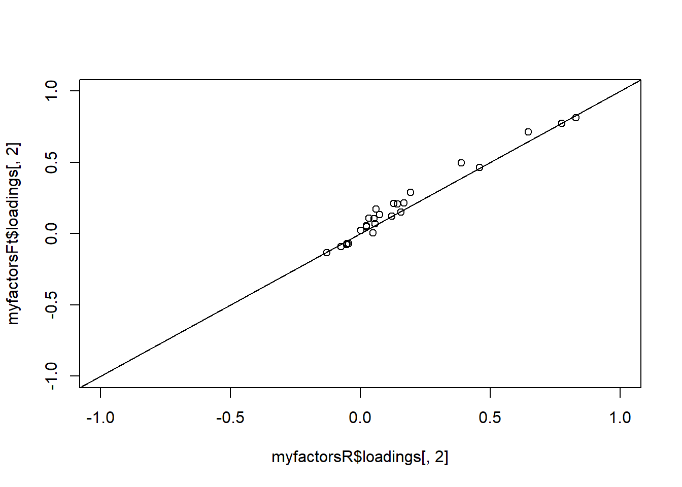
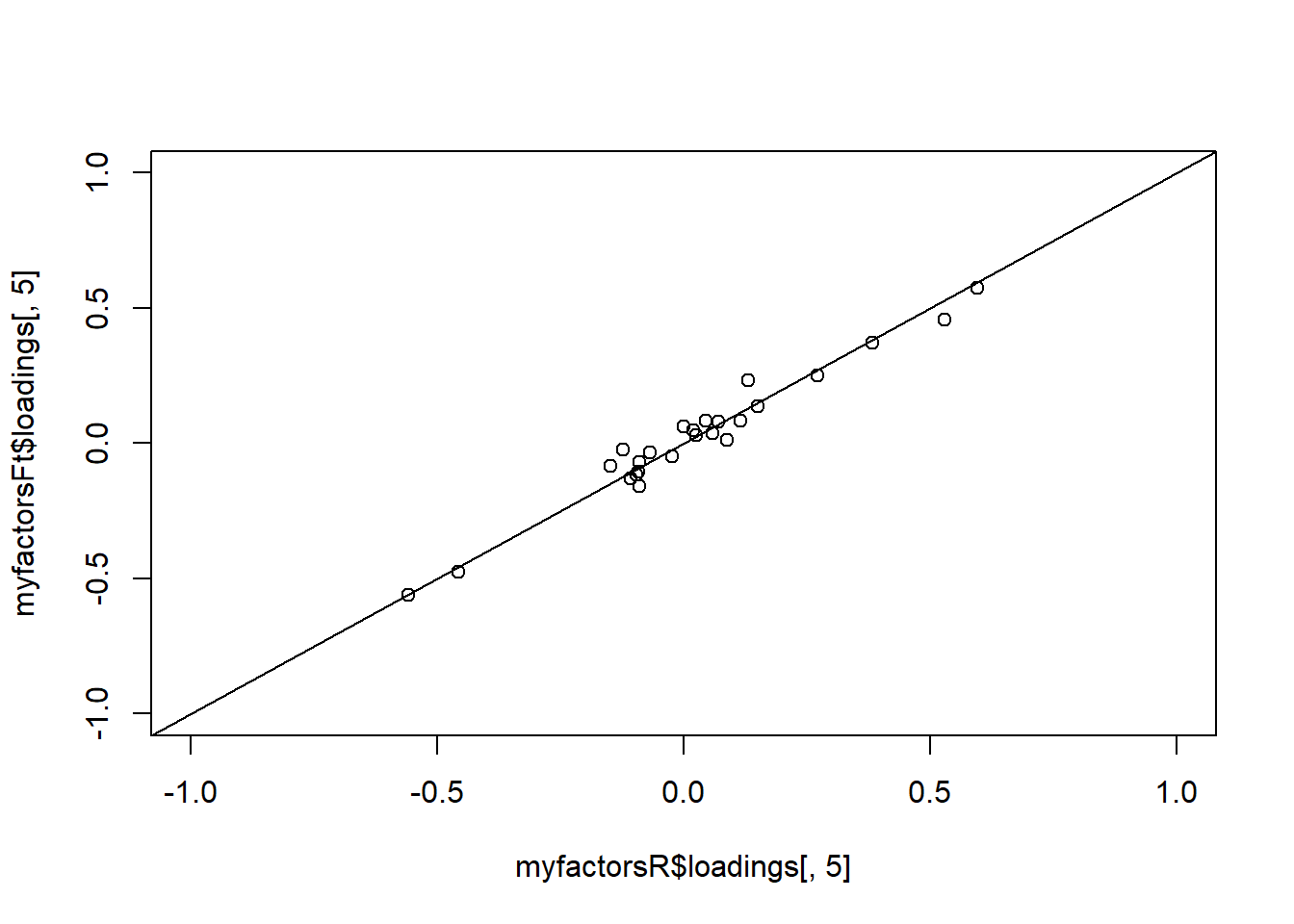
In this respect it is useful to plot the factor loadings of corresponding factors across the two groups and to compare it to an identity line (that represents perfect correspondence). An advantage of the plot is that it can highlight particular variables that have different factor loadings.

Scatter plots of corresponding factors

In the plots below we see that the factors manifested very similarly across the two groups. It is noticeable that the factor loadings for Extroversion show greater dispersion around the identity line than the remaining factors.

plot(myfactorsR$loadings[, 1], 
     myfactorsFt$loadings[, 1], 
     xlim = c(-1, 1), 
     ylim = c(-1, 1))

abline(0, 1)

plot(myfactorsR$loadings[, 2], 
     myfactorsFt$loadings[, 2], 
     xlim = c(-1, 1), 
     ylim = c(-1, 1))

abline(0, 1)

plot(myfactorsR$loadings[, 3], 
     myfactorsFt$loadings[, 3], 
     xlim = c(-1, 1), 
     ylim = c(-1, 1))

abline(0, 1)

plot(myfactorsR$loadings[, 4], 
     myfactorsFt$loadings[, 4], 
     xlim = c(-1, 1), 
     ylim = c(-1, 1))

abline(0, 1)

plot(myfactorsR$loadings[, 5], 
     myfactorsFt$loadings[, 5], 
     xlim = c(-1, 1), 
     ylim = c(-1, 1))

abline(0, 1)

The root mean square difference of factor loadings

The overall similarities of the factors can also be expressed with reference to differences in the size of the corresponding factor loadings across the two groups. In this respect the root of the mean squared difference (RMSD) of the corresponding factor loadings reflects the average size of the differences.

In our example the RMSDs of the Extroversion and Agreeableness factors were slightly higher than those of the remaining factors. These were also the factors that had the lowest coefficients of congruence.

sqrt(mean((myfactorsR$loadings[, 1] - myfactorsFt$loadings[, 1])^2))
[1] 0.103
sqrt(mean((myfactorsR$loadings[, 2] - myfactorsFt$loadings[, 2])^2))
[1] 0.0524
sqrt(mean((myfactorsR$loadings[, 3] - myfactorsFt$loadings[, 3])^2))
[1] 0.0788
sqrt(mean((myfactorsR$loadings[, 4] - myfactorsFt$loadings[, 4])^2))
[1] 0.0433
sqrt(mean((myfactorsR$loadings[, 5] - myfactorsFt$loadings[, 5])^2))
[1] 0.046

References

Lorenzo-Seva, U. & ten Berge, J. M. F. (2006). Methodology, 2(2), 57:64. doi: 10.1027/1614-1881.2.2.57

Revelle, W. (2024a). psych: Procedures for psychological, psychometric, and personality research. Northwestern University, Evanston, Illinois. R package version 2.4.6, https://CRAN.R-project.org/package=psych.

Revelle, W. (2024b). psychTools: Tools to accompany the ‘psych’ package for psychological research. Northwestern University, Evanston, Illinois. R package version 2.4.3, https://CRAN.R-project.org/package=psychTools.