      x1    x2    x3    y1    y2    y3    z1   z2    z3
1   2.43  1.36  1.41  1.45  0.96  1.21  0.82 1.61  0.94
2   0.25  0.27  0.58  0.55  0.71 -0.14  3.66 2.61  3.15
3  -1.36 -0.56 -0.10 -0.98 -0.67  0.01  1.72 2.11  0.91
4   3.04  2.22  1.61  6.46  4.78  5.99  2.57 3.26  3.39
5   2.81  2.70  2.58  2.29  2.15  1.55  0.35 0.07 -0.02
6  -0.55 -0.75 -0.64  1.13  1.20  0.36 -0.24 0.60  0.32
7  -0.38  0.44  0.64  0.18  0.02 -0.17  1.21 1.19  1.58
8   0.31  0.44 -0.13  1.10  0.27  0.50  0.66 0.74  0.43
9   0.93  1.99  1.14 -0.46  0.70  0.67  1.44 1.78  1.70
10  0.60  1.10  0.41 -0.11 -0.31 -0.86 -0.13 0.51 -0.04
The modsem package
Kjell Slupphaug recently published the modsem package for R. The package can be used to test hypotheses about moderation (interactions) with latent variables.
I give two brief examples below to demonstrate how to implement (a) Marsh’s double mean centering approach, and (b) Little’s residual centering approach. The package offers several other approaches, but these two are very popular.
These examples come from the help pages of the package. They are very simple, but the modsem package can deal with very complex models where the moderating effects are embedded in bigger models. One can even model interactions of endogenous latent variables without difficulty. The package has several “vignettes” that provide more detail. Also check out his description of the modsem package here: https://bookdown.org/slupphaugkjell/quartomodsem/
Here is a nice video of how to examine latent interactions via Marsh’s double-mean centering approach: https://www.youtube.com/watch?v=gAV2fmHrPPw. Note that this video was made before the modsem package became available. It is now much easier to do the analysis and far less coding is required. What is nice about the video is that it more clearly shows the logic of what is happening when testing for latent interactions.
The data
I use a built in data set of the modsem package, namely oneInt. There are nine manifest variables: x1, x2 and x3 are indicators of latent variable X, z1, z2 and z3 are indicators of latent variable Z, and y1,y2 and y3 are indicators of latent variable Y. X is the focal independent variable, Y is the dependent variable and Z is the presumed moderator.
Here are the observed data of the first 10 people. There are no product terms of observed indicators. This will be taken care of by the modsem package.
The structural model
The basic structural model without the moderating effect looks as follows. In the first part we define the latent variables using the =~ operator. In the second part we define the actual structural model with the ~ operator.
model1 <- '
X =~ x1 + x2 + x3
Z =~ z1 + z2 + z3
Y =~ y1 + y2 + y3

Y ~ X + Z
'
The structural model with the latent moderating effect looks as follows. We simply add the effect by including X:Z in the structural model. There is no need to include the definition of the latent interaction factor.
model2 <- '
X =~ x1 + x2 + x3
Z =~ z1 + z2 + z3
Y =~ y1 + y2 + y3

Y ~ X + Z + X:Z
'
Activating the packages we will need
library(lavaan)
library(modsem)
Fitting the model to the observed data with double mean centering
We employ the modsem function to fit the model to the data. There is a lot of output. Here we focus on the regression of Y on XZ (the moderating effect). If we scroll down through the output to the section with the header “Regressions” we note the that partial regression coefficient is statistically significant, \(b_3 = 0.702, z = 26.360, p < 0.001\), which means that Z does moderate the effect of X on Y. As an aside, if you examine the section with the header “Covariances” you will note at the bottom that the covariances of X and Z with the interaction term XZ are close to zero (which is the purpose of the double mean centering approach).
fit.Marsh <- modsem(model2,
                    data   = oneInt,
                    method = "dblcent")

summary(fit.Marsh,
        standardized = TRUE,
        fit.measures = TRUE)
modsem:
Method = dblcent lavaan 0.6-19 ended normally after 157 iterations
Estimator ML
Optimization method NLMINB
Number of model parameters 60
Number of observations 2000
Model Test User Model:
Test statistic 122.924
Degrees of freedom 111
P-value (Chi-square) 0.207
Model Test Baseline Model:
Test statistic 51898.582
Degrees of freedom 153
P-value 0.000
User Model versus Baseline Model:
Comparative Fit Index (CFI) 1.000
Tucker-Lewis Index (TLI) 1.000
Loglikelihood and Information Criteria:
Loglikelihood user model (H0) -26807.612
Loglikelihood unrestricted model (H1) -26746.150
Akaike (AIC) 53735.224
Bayesian (BIC) 54071.279
Sample-size adjusted Bayesian (SABIC) 53880.655
Root Mean Square Error of Approximation:
RMSEA 0.007
90 Percent confidence interval - lower 0.000
90 Percent confidence interval - upper 0.014
P-value H_0: RMSEA <= 0.050 1.000
P-value H_0: RMSEA >= 0.080 0.000
Standardized Root Mean Square Residual:
SRMR 0.008
Parameter Estimates:
Standard errors Standard
Information Expected
Information saturated (h1) model Structured
Latent Variables:
Estimate Std.Err z-value P(>|z|) Std.lv Std.all
X =~
x1 1.000 0.990 0.927
x2 0.804 0.013 63.612 0.000 0.796 0.892
x3 0.916 0.014 67.144 0.000 0.907 0.914
Z =~
z1 1.000 1.008 0.926
z2 0.812 0.013 64.763 0.000 0.818 0.899
z3 0.882 0.013 67.014 0.000 0.889 0.913
Y =~
y1 1.000 1.577 0.969
y2 0.798 0.007 107.428 0.000 1.259 0.955
y3 0.899 0.008 112.453 0.000 1.418 0.962
XZ =~
x1z1 1.000 1.022 0.878
x2z1 0.805 0.013 60.636 0.000 0.823 0.836
x3z1 0.877 0.014 62.680 0.000 0.897 0.843
x1z2 0.793 0.013 59.343 0.000 0.810 0.833
x2z2 0.646 0.015 43.672 0.000 0.661 0.804
x3z2 0.706 0.016 44.292 0.000 0.722 0.812
x1z3 0.887 0.014 63.700 0.000 0.907 0.867
x2z3 0.716 0.016 45.645 0.000 0.732 0.829
x3z3 0.781 0.017 45.339 0.000 0.799 0.826
Regressions:
Estimate Std.Err z-value P(>|z|) Std.lv Std.all
Y ~
X 0.675 0.027 25.379 0.000 0.424 0.424
Z 0.561 0.026 21.606 0.000 0.358 0.358
XZ 0.702 0.027 26.360 0.000 0.455 0.455
Covariances:
Estimate Std.Err z-value P(>|z|) Std.lv Std.all
.x1z1 ~~
.x2z2 0.000 0.000 0.000
.x2z3 0.000 0.000 0.000
.x3z2 0.000 0.000 0.000
.x3z3 0.000 0.000 0.000
.x2z1 ~~
.x1z2 0.000 0.000 0.000
.x1z2 ~~
.x2z3 0.000 0.000 0.000
.x3z1 ~~
.x1z2 0.000 0.000 0.000
.x1z2 ~~
.x3z3 0.000 0.000 0.000
.x2z1 ~~
.x1z3 0.000 0.000 0.000
.x2z2 ~~
.x1z3 0.000 0.000 0.000
.x3z1 ~~
.x1z3 0.000 0.000 0.000
.x3z2 ~~
.x1z3 0.000 0.000 0.000
.x2z1 ~~
.x3z2 0.000 0.000 0.000
.x3z3 0.000 0.000 0.000
.x3z1 ~~
.x2z2 0.000 0.000 0.000
.x2z2 ~~
.x3z3 0.000 0.000 0.000
.x3z1 ~~
.x2z3 0.000 0.000 0.000
.x3z2 ~~
.x2z3 0.000 0.000 0.000
.x1z1 ~~
.x1z2 0.115 0.008 14.802 0.000 0.115 0.384
.x1z3 0.114 0.008 13.947 0.000 0.114 0.393
.x2z1 0.125 0.008 16.095 0.000 0.125 0.415
.x3z1 0.140 0.009 16.135 0.000 0.140 0.440
.x1z2 ~~
.x1z3 0.103 0.007 14.675 0.000 0.103 0.367
.x2z2 0.128 0.006 20.850 0.000 0.128 0.486
.x3z2 0.146 0.007 21.243 0.000 0.146 0.520
.x1z3 ~~
.x2z3 0.116 0.007 17.818 0.000 0.116 0.450
.x3z3 0.135 0.007 18.335 0.000 0.135 0.474
.x2z1 ~~
.x2z2 0.135 0.006 20.905 0.000 0.135 0.510
.x2z3 0.145 0.007 21.145 0.000 0.145 0.542
.x3z1 0.114 0.007 16.058 0.000 0.114 0.370
.x2z2 ~~
.x2z3 0.117 0.006 20.419 0.000 0.117 0.486
.x3z2 0.116 0.006 20.586 0.000 0.116 0.456
.x2z3 ~~
.x3z3 0.109 0.006 18.059 0.000 0.109 0.404
.x3z1 ~~
.x3z2 0.138 0.007 19.331 0.000 0.138 0.464
.x3z3 0.158 0.008 20.269 0.000 0.158 0.507
.x3z2 ~~
.x3z3 0.131 0.007 19.958 0.000 0.131 0.464
X ~~
Z 0.201 0.024 8.271 0.000 0.201 0.201
XZ 0.016 0.025 0.628 0.530 0.015 0.015
Z ~~
XZ 0.062 0.025 2.449 0.014 0.060 0.060
Variances:
Estimate Std.Err z-value P(>|z|) Std.lv Std.all
.x1 0.160 0.009 17.871 0.000 0.160 0.140
.x2 0.162 0.007 22.969 0.000 0.162 0.204
.x3 0.163 0.008 20.161 0.000 0.163 0.165
.z1 0.168 0.009 18.143 0.000 0.168 0.142
.z2 0.158 0.007 22.264 0.000 0.158 0.191
.z3 0.158 0.008 20.389 0.000 0.158 0.167
.y1 0.159 0.009 17.896 0.000 0.159 0.060
.y2 0.154 0.007 22.640 0.000 0.154 0.089
.y3 0.164 0.008 20.698 0.000 0.164 0.075
.x1z1 0.311 0.014 22.227 0.000 0.311 0.229
.x2z1 0.292 0.011 27.287 0.000 0.292 0.301
.x3z1 0.327 0.012 26.275 0.000 0.327 0.289
.x1z2 0.290 0.011 26.910 0.000 0.290 0.306
.x2z2 0.239 0.008 29.770 0.000 0.239 0.353
.x3z2 0.270 0.009 29.117 0.000 0.270 0.341
.x1z3 0.272 0.012 23.586 0.000 0.272 0.249
.x2z3 0.245 0.009 27.979 0.000 0.245 0.313
.x3z3 0.297 0.011 28.154 0.000 0.297 0.317
X 0.981 0.036 26.895 0.000 1.000 1.000
Z 1.016 0.038 26.856 0.000 1.000 1.000
.Y 0.990 0.038 25.926 0.000 0.398 0.398
XZ 1.045 0.044 24.004 0.000 1.000 1.000Plotting the interaction
To gain insight into the nature of the moderating effect it is useful to plot the simple slopes of X at different levels of Z. We employ the plot_interaction() function for this purpose: we specify as arguments the names of the latent variables, the limits of the x-axis on the plot, the values of Z for which we want to find the simple slopes of X and the name of the fitted model. It is common to find the simple slopes of X at one standard deviation below the mean of Z, at the mean of Z, and one standard deviation above the mean of Z. The output of the fitted model shows the estimated variance of Z (almost right at the bottom of the output) to be 1.016. The standard deviation is the square root of the variance.
plot_interaction("X",
                 "Z",
                 "Y",
                 "XZ",
                 vals_x = c(-3, 3),
                 vals_z = c(-sqrt(1.016), 0, sqrt(1.016)),
                 fit.Marsh)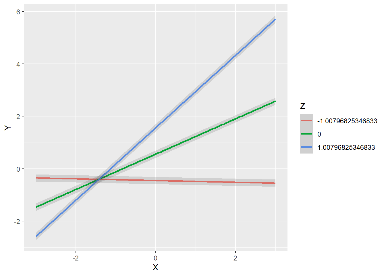
Fitting the model to the observed data with residual centering
We again employ the modsem function to fit the model to the data, but we change the method to "rca". The partial regression coefficient of the interaction term, XZ, is almost identical to what we found with the double mean centered method: \(b_3 = 0.704, z = 26.401, p < 0.001\). Note that the covariances of X and Z with the interaction term XZ are now exactly zero (which again is the purpose of the residual centering approach).
fit.Little <- modsem(model2,
                     data   = oneInt,
                     method = "rca")

summary(fit.Little,
        standardized = TRUE,
        fit.measures = TRUE)
modsem:
Method = rca lavaan 0.6-19 ended normally after 174 iterations
Estimator ML
Optimization method NLMINB
Number of model parameters 60
Number of observations 2000
Model Test User Model:
Test statistic 39.277
Degrees of freedom 111
P-value (Chi-square) 1.000
Model Test Baseline Model:
Test statistic 51813.975
Degrees of freedom 153
P-value 0.000
User Model versus Baseline Model:
Comparative Fit Index (CFI) 1.000
Tucker-Lewis Index (TLI) 1.002
Loglikelihood and Information Criteria:
Loglikelihood user model (H0) -26765.789
Loglikelihood unrestricted model (H1) -26746.150
Akaike (AIC) 53651.578
Bayesian (BIC) 53987.632
Sample-size adjusted Bayesian (SABIC) 53797.008
Root Mean Square Error of Approximation:
RMSEA 0.000
90 Percent confidence interval - lower 0.000
90 Percent confidence interval - upper 0.000
P-value H_0: RMSEA <= 0.050 1.000
P-value H_0: RMSEA >= 0.080 0.000
Standardized Root Mean Square Residual:
SRMR 0.004
Parameter Estimates:
Standard errors Standard
Information Expected
Information saturated (h1) model Structured
Latent Variables:
Estimate Std.Err z-value P(>|z|) Std.lv Std.all
X =~
x1 1.000 0.990 0.927
x2 0.804 0.013 63.620 0.000 0.797 0.893
x3 0.916 0.014 67.138 0.000 0.907 0.914
Z =~
z1 1.000 1.008 0.926
z2 0.812 0.013 64.688 0.000 0.818 0.899
z3 0.883 0.013 67.116 0.000 0.890 0.914
Y =~
y1 1.000 1.577 0.969
y2 0.798 0.007 107.434 0.000 1.259 0.955
y3 0.899 0.008 112.454 0.000 1.418 0.962
XZ =~
x1z1 1.000 1.020 0.878
x2z1 0.806 0.013 60.667 0.000 0.822 0.837
x3z1 0.877 0.014 62.578 0.000 0.894 0.843
x1z2 0.792 0.013 59.420 0.000 0.808 0.833
x2z2 0.646 0.015 43.626 0.000 0.659 0.804
x3z2 0.707 0.016 44.285 0.000 0.721 0.812
x1z3 0.886 0.014 63.629 0.000 0.904 0.866
x2z3 0.717 0.016 45.633 0.000 0.731 0.829
x3z3 0.781 0.017 45.316 0.000 0.797 0.826
Regressions:
Estimate Std.Err z-value P(>|z|) Std.lv Std.all
Y ~
X 0.677 0.027 25.454 0.000 0.425 0.425
Z 0.603 0.026 23.192 0.000 0.385 0.385
XZ 0.704 0.027 26.401 0.000 0.455 0.455
Covariances:
Estimate Std.Err z-value P(>|z|) Std.lv Std.all
.x1z1 ~~
.x2z2 0.000 0.000 0.000
.x2z3 0.000 0.000 0.000
.x3z2 0.000 0.000 0.000
.x3z3 0.000 0.000 0.000
.x2z1 ~~
.x1z2 0.000 0.000 0.000
.x1z2 ~~
.x2z3 0.000 0.000 0.000
.x3z1 ~~
.x1z2 0.000 0.000 0.000
.x1z2 ~~
.x3z3 0.000 0.000 0.000
.x2z1 ~~
.x1z3 0.000 0.000 0.000
.x2z2 ~~
.x1z3 0.000 0.000 0.000
.x3z1 ~~
.x1z3 0.000 0.000 0.000
.x3z2 ~~
.x1z3 0.000 0.000 0.000
.x2z1 ~~
.x3z2 0.000 0.000 0.000
.x3z3 0.000 0.000 0.000
.x3z1 ~~
.x2z2 0.000 0.000 0.000
.x2z2 ~~
.x3z3 0.000 0.000 0.000
.x3z1 ~~
.x2z3 0.000 0.000 0.000
.x3z2 ~~
.x2z3 0.000 0.000 0.000
.x1z1 ~~
.x1z2 0.116 0.008 14.905 0.000 0.116 0.387
.x1z3 0.115 0.008 14.064 0.000 0.115 0.395
.x2z1 0.124 0.008 16.064 0.000 0.124 0.414
.x3z1 0.139 0.009 16.102 0.000 0.139 0.438
.x1z2 ~~
.x1z3 0.103 0.007 14.763 0.000 0.103 0.369
.x2z2 0.127 0.006 20.848 0.000 0.127 0.486
.x3z2 0.144 0.007 21.203 0.000 0.144 0.519
.x1z3 ~~
.x2z3 0.116 0.006 17.846 0.000 0.116 0.450
.x3z3 0.135 0.007 18.404 0.000 0.135 0.475
.x2z1 ~~
.x2z2 0.134 0.006 20.854 0.000 0.134 0.509
.x2z3 0.144 0.007 21.081 0.000 0.144 0.541
.x3z1 0.114 0.007 16.018 0.000 0.114 0.370
.x2z2 ~~
.x2z3 0.117 0.006 20.390 0.000 0.117 0.486
.x3z2 0.115 0.006 20.591 0.000 0.115 0.456
.x2z3 ~~
.x3z3 0.108 0.006 18.066 0.000 0.108 0.405
.x3z1 ~~
.x3z2 0.137 0.007 19.301 0.000 0.137 0.464
.x3z3 0.157 0.008 20.231 0.000 0.157 0.506
.x3z2 ~~
.x3z3 0.130 0.007 19.906 0.000 0.130 0.463
X ~~
Z 0.201 0.024 8.270 0.000 0.201 0.201
XZ 0.000 0.025 0.000 1.000 0.000 0.000
Z ~~
XZ 0.000 0.025 0.000 1.000 0.000 0.000
Variances:
Estimate Std.Err z-value P(>|z|) Std.lv Std.all
.x1 0.160 0.009 17.885 0.000 0.160 0.140
.x2 0.162 0.007 22.962 0.000 0.162 0.203
.x3 0.163 0.008 20.166 0.000 0.163 0.165
.z1 0.169 0.009 18.277 0.000 0.169 0.143
.z2 0.159 0.007 22.326 0.000 0.159 0.192
.z3 0.157 0.008 20.310 0.000 0.157 0.165
.y1 0.159 0.009 17.889 0.000 0.159 0.060
.y2 0.154 0.007 22.641 0.000 0.154 0.089
.y3 0.164 0.008 20.702 0.000 0.164 0.075
.x1z1 0.310 0.014 22.272 0.000 0.310 0.230
.x2z1 0.290 0.011 27.205 0.000 0.290 0.300
.x3z1 0.325 0.012 26.241 0.000 0.325 0.289
.x1z2 0.289 0.011 26.924 0.000 0.289 0.307
.x2z2 0.238 0.008 29.764 0.000 0.238 0.354
.x3z2 0.268 0.009 29.072 0.000 0.268 0.340
.x1z3 0.273 0.011 23.699 0.000 0.273 0.250
.x2z3 0.243 0.009 27.945 0.000 0.243 0.313
.x3z3 0.295 0.010 28.140 0.000 0.295 0.317
X 0.981 0.036 26.893 0.000 1.000 1.000
Z 1.015 0.038 26.835 0.000 1.000 1.000
.Y 0.988 0.038 25.838 0.000 0.397 0.397
XZ 1.041 0.043 23.988 0.000 1.000 1.000Plotting the interaction
plot_interaction("X",
                 "Z",
                 "Y",
                 "XZ",
                 vals_x = c(-3, 3),
                 vals_z = c(-sqrt(1.015), 0, sqrt(1.015)),
                 fit.Little)