Introduction
This document contains a basic example of how one might fit an exploratory structural equation model (esem) with the lavaan package in R. A structural equation model (sem) usually consists of two parts: (a) a measurement model, and (b) a structural model. The measurement model typically is a confirmatory factor analysis model that specifies which clusters of items serve as indicators of which factors. Sometimes researchers may be unable to specify such a model beforehand, or such a model may be deemed too restrictive (for instance, some personality researchers argue that personality measures are too complex to fit simple restrictive confirmatory factor analysis models). In such cases, an analyst can choose to fit an unrestricted exploratory factor analysis model. In contrast to confirmatory factor analysis, the nature of the factors are not specified beforehand. Rather, in an exploratory factor analysis the analyst “allows the data to speak”. The factors that emerge from the analysis are interpreted by focusing on the pattern of the indicators that have strong and weak factor loadings.
In a standard sem analysis the factors are “defined” by the measurement model and they are then employed in a structural model that specifies relations between the latent variables. In an esem analysis the factors are “found” and they are then further employed in a structural model.
Explaining variance in education by means of the big five personality factors
I demonstrate three approaches to explaining variance in education by means of the big five personality factors. First, I obtain factor scores of the big five with an exploratory factor analysis. These observed scores are then used in a multiple regression analysis, where education is the dependent variable and the five traits are the independent variables.
Second, I perform a standard sem analysis, where there the five factors are estimated via confirmatory factor analysis and education is then regressed on the factors. This is the standard approach that most analysts would employ.
Third, I perform an exploratory structural equation modeling analysis, where the five factors are obtained via exploratory factor analysis and education is then then regressed on five factors. This is an approach that would appeal to some personality psychologists who argue that personality variables are too complex to fit simple independent clusters confirmatory factor analysis models.
Below I give visual depictions of the standardized results of the three approaches.
Multiple regression analysis
Structural equation modeling analysis
Exploratory structural equation modeling analysis
Simple multiple regression analysis using the factor scores of an EFA
Readers who are only interested in the esem analysis can skip to page 13.
The data
I employ the bfi dataset that is included in the psychTools package. It contains the responses of 2800 persons to the 25 items of the Big Five Inventory. It also contains a variable education that reflect the participants’ educational levels: 1 = High school, 2 = Finished high school, 3 = some college, 4 = college graduate, and 5 = graduate degree. Whereas it is clearly an ordinal variable, I treat it here as if it is continuous.
There are several variables that need to be reverse scored if total scores are calculated. Strictly, it is not necessary to reverse score items for a factor analysis or sem analysis. However, to avoid potential confusion I reverse scored all the items such that they are now all scored in the direction of the factor name (e.g. higher scores on all the Agreeableness items indicate higher Agreeableness). I stored the recoded items along with the education variable in a data frame labelled bfi.data. This is the dataset that is further analysed.
library(psychTools)
library(psych)
data(bfi)
### Reverse scoring the items
keys <-  c(-1, 1, 1, 1, 1,
            1, 1, 1,-1,-1,
           -1,-1, 1, 1, 1,
            1, 1, 1, 1, 1,
            1,-1, 1, 1,-1)

bfi.data <- reverse.code(keys, bfi[1:25])
bfi.data <- cbind(bfi.data, bfi$education)
colnames(bfi.data) <- colnames(bfi[c(1:25, 27)])
bfi.data <- data.frame(bfi.data)
As a baseline, I performed an exploratory factor analysis of the 25 items of the bfi. I specified five factors and rotate them according to the popular “Direct Oblimin” criterion, which yields correlated (oblique) factors. I obtained for each person a factor score according to tenBerge’s method. This method yields observed factor scores that retain the correlations of the obliquely rotated latent factors.
I renamed the factors to correspond with the names of the big five traits (after inspection of the rotated factor matrix): MR2 = Neuroticism (Nfac), MR1 = Extroversion (Efac), MR3 = Conscientiousness (Cfac, MR5 = Agreeableness (Afac), and MR4 = Openness (Ofac). I then added these factor scores to the dataset. Note that in place of the factor scores I could have used simple summated total scores of the five personality subscales.
myfa <- psych::fa(bfi.data[1:25],
                  nfactors = 5,
                  rotate = "oblimin",
                  scores = "tenBerge")

print(myfa, cut = 0.30)
Factor Analysis using method = minres
Call: psych::fa(r = bfi.data[1:25], nfactors = 5, rotate = "oblimin",
scores = "tenBerge")
Standardized loadings (pattern matrix) based upon correlation matrix
MR2 MR1 MR3 MR5 MR4 h2 u2 com
A1 0.41 0.19 0.81 2.0
A2 0.64 0.45 0.55 1.0
A3 0.66 0.52 0.48 1.1
A4 0.43 0.28 0.72 1.7
A5 0.53 0.46 0.54 1.5
C1 0.55 0.33 0.67 1.2
C2 0.67 0.45 0.55 1.2
C3 0.57 0.32 0.68 1.1
C4 0.61 0.45 0.55 1.2
C5 0.55 0.43 0.57 1.4
E1 0.56 0.35 0.65 1.2
E2 0.68 0.54 0.46 1.1
E3 0.42 0.44 0.56 2.6
E4 0.59 0.53 0.47 1.5
E5 0.42 0.40 0.60 2.6
N1 0.81 0.65 0.35 1.1
N2 0.78 0.60 0.40 1.0
N3 0.71 0.55 0.45 1.1
N4 0.47 -0.39 0.49 0.51 2.3
N5 0.49 0.35 0.65 2.0
O1 0.51 0.31 0.69 1.1
O2 0.46 0.26 0.74 1.7
O3 0.61 0.46 0.54 1.2
O4 -0.32 0.37 0.25 0.75 2.7
O5 0.54 0.30 0.70 1.2
MR2 MR1 MR3 MR5 MR4
SS loadings 2.57 2.20 2.03 1.99 1.59
Proportion Var 0.10 0.09 0.08 0.08 0.06
Cumulative Var 0.10 0.19 0.27 0.35 0.41
Proportion Explained 0.25 0.21 0.20 0.19 0.15
Cumulative Proportion 0.25 0.46 0.66 0.85 1.00
With factor correlations of
MR2 MR1 MR3 MR5 MR4
MR2 1.00 -0.21 -0.19 -0.04 -0.01
MR1 -0.21 1.00 0.23 0.33 0.17
MR3 -0.19 0.23 1.00 0.20 0.19
MR5 -0.04 0.33 0.20 1.00 0.19
MR4 -0.01 0.17 0.19 0.19 1.00
Mean item complexity = 1.5
Test of the hypothesis that 5 factors are sufficient.
df null model = 300 with the objective function = 7.23 with Chi Square = 20163.79
df of the model are 185 and the objective function was 0.65
The root mean square of the residuals (RMSR) is 0.03
The df corrected root mean square of the residuals is 0.04
The harmonic n.obs is 2762 with the empirical chi square 1392.16 with prob < 5.6e-184
The total n.obs was 2800 with Likelihood Chi Square = 1808.94 with prob < 4.3e-264
Tucker Lewis Index of factoring reliability = 0.867
RMSEA index = 0.056 and the 90 % confidence intervals are 0.054 0.058
BIC = 340.53
Fit based upon off diagonal values = 0.98
Measures of factor score adequacy
MR2 MR1 MR3 MR5 MR4
Correlation of (regression) scores with factors 0.92 0.89 0.88 0.88 0.84
Multiple R square of scores with factors 0.85 0.79 0.77 0.77 0.71
Minimum correlation of possible factor scores 0.70 0.59 0.54 0.54 0.42colnames(myfa$scores) <- c("Nfac", "Efac", "Cfac", "Afac", "Ofac")
bfi.data <- cbind(bfi.data, myfa$scores)Multiple regression of education on the big five factors
Next, I performed a simple multiple regression analysis, where the five factors are the independent variables and education is the dependent variable. Note that the observed factor scores are not free of measurement error. Results show that the five factors jointly accounted for about 2% of the variance in education: \(R^2 = 0.0197\). The partial regression coefficients of Nfac (\(b_1 = -0.06, t = -2.63, p = 0.009\)), Efac (\(b_2 = -0.07, t = -2.76, p = 0.006\)), and Ofac (\(b_5 = 0.14, t = 5.84, p < 0.001\)) were statistically significant.
These results show that education is positively (but weakly) related to Openness,and negatively (but weakly) related to Extroversion and Neuroticism.
m1 <- lm(education ~ Nfac + Efac + Cfac + Afac + Ofac, data = bfi.data)
summary(m1)
Call:
lm(formula = education ~ Nfac + Efac + Cfac + Afac + Ofac, data = bfi.data)

Residuals:
    Min      1Q  Median      3Q     Max
-2.6442 -0.3592 -0.1179  0.7563  2.1918

Coefficients:
             Estimate Std. Error t value Pr(>|t|)
(Intercept)  3.183996   0.023349 136.367  < 2e-16 ***
Nfac        -0.063580   0.024198  -2.627  0.00866 **
Efac        -0.071267   0.025860  -2.756  0.00590 **
Cfac         0.003952   0.024753   0.160  0.87315
Afac         0.025187   0.025338   0.994  0.32032
Ofac         0.140786   0.024128   5.835 6.17e-09 ***
---
Signif. codes:  0 '***' 0.001 '**' 0.01 '*' 0.05 '.' 0.1 ' ' 1

Residual standard error: 1.102 on 2230 degrees of freedom
  (564 observations deleted due to missingness)
Multiple R-squared:  0.01967,   Adjusted R-squared:  0.01747
F-statistic: 8.948 on 5 and 2230 DF,  p-value: 1.987e-08
Fitting the multiple regression model in lavaan
Multiple regression analyses are typically performed using ordinary least squares. However, it is possible to do the analysis with sem software, in which case the parameters can be estimated with a wide variety of estimators, of which maximum likelihood is the most popular.
Here I demonstrate how the analysis can be done in lavaan, using robust maximum likelihood. The results of this analysis and the standard multiple regression are virtually the same.
library(lavaan)

reg.model <- '
education ~ Afac + Cfac + Efac + Nfac + Ofac
'

fit.reg.model <- sem(reg.model,
                     data      = bfi.data,
                     estimator = "MLR")

summary(fit.reg.model,
        standardized = TRUE,
        rsquare      = TRUE)
lavaan 0.6-19 ended normally after 1 iteration
Estimator ML
Optimization method NLMINB
Number of model parameters 6
Used Total
Number of observations 2236 2800
Model Test User Model:
Standard Scaled
Test Statistic 0.000 0.000
Degrees of freedom 0 0
Parameter Estimates:
Standard errors Sandwich
Information bread Observed
Observed information based on Hessian
Regressions:
Estimate Std.Err z-value P(>|z|) Std.lv Std.all
education ~
Afac 0.025 0.025 0.990 0.322 0.025 0.022
Cfac 0.004 0.026 0.153 0.879 0.004 0.004
Efac -0.071 0.026 -2.743 0.006 -0.071 -0.064
Nfac -0.064 0.023 -2.720 0.007 -0.064 -0.057
Ofac 0.141 0.025 5.665 0.000 0.141 0.126
Variances:
Estimate Std.Err z-value P(>|z|) Std.lv Std.all
.education 1.211 0.034 35.983 0.000 1.211 0.980
R-Square:
Estimate
education 0.020Regression of education on the big five with latent factors (sem analysis)
Next, we examine the effect of the big five factors on education within a standard structural equation modeling framework. We treat the big five as latent variables and education as a manifest variable. The indicators of the big five factors are the items of the Big Five Inventory.
Note that the measurement model forces a strict independent clusters model, where for each item a loading is estimated on one factor, and the loadings on the remaining factors are fixed to zero. For instance, the loading of item A1 on the Agreeableness factor is estimated, but its loadings on the remaining big five factors are fixed to zero.
The five personality factors in this model are labelled E.cfa, A.cfa, N.cfa, O.cfa, and C.cfa. The structural model specifies these five factors as independent variables and education as the dependent variable.
This model fitted the data poorly: robust CFI = 0.78, robust TLI = 0.75, robust RMSEA = 0.075, SRMR = 0.074. One might now turn to modification indices and inspection of the residuals to identify the sources of the misfit. As stated earlier, some personality psychologists would argue that because of the complexity of personality, the independent clusters measurement model was doomed to failure before the analysis began.
The five factors jointly accounted for 2.3% of the variance in education: \(R^2 = 0.023\). The regression coefficients of E.cfa (\(b_3 = -0.128, z = -2.277, p = 0.023\)) and O.cfa (\(b_5 = 0.288, z = 4.81, p < 0.001\)) were statistically significant. Given the poor fit of the model it is not clear how much confidence we can have in these parameter estimates.
library(lavaan)
sem.model <- '

A.cfa =~ A1 + A2 + A3 + A4 + A5
C.cfa =~ C1 + C2 + C3 + C4 + C5
E.cfa =~ E1 + E2 + E3 + E4 + E5
N.cfa =~ N1 + N2 + N3 + N4 + N5
O.cfa =~ O1 + O2 + O3 + O4 + O5

education ~ A.cfa + C.cfa + E.cfa + N.cfa + O.cfa
'

fit.sem.model <- sem(sem.model,
                     data      = bfi.data,
                     estimator = "MLR")

summary(fit.sem.model,
        standardized = TRUE,
        fit.measures = TRUE,
        rsquare      = TRUE)
lavaan 0.6-19 ended normally after 57 iterations
Estimator ML
Optimization method NLMINB
Number of model parameters 66
Used Total
Number of observations 2236 2800
Model Test User Model:
Standard Scaled
Test Statistic 3930.086 3436.167
Degrees of freedom 285 285
P-value (Chi-square) 0.000 0.000
Scaling correction factor 1.144
Yuan-Bentler correction (Mplus variant)
Model Test Baseline Model:
Test statistic 16679.316 14146.038
Degrees of freedom 325 325
P-value 0.000 0.000
Scaling correction factor 1.179
User Model versus Baseline Model:
Comparative Fit Index (CFI) 0.777 0.772
Tucker-Lewis Index (TLI) 0.746 0.740
Robust Comparative Fit Index (CFI) 0.779
Robust Tucker-Lewis Index (TLI) 0.748
Loglikelihood and Information Criteria:
Loglikelihood user model (H0) -94682.026 -94682.026
Scaling correction factor 1.209
for the MLR correction
Loglikelihood unrestricted model (H1) -92716.983 -92716.983
Scaling correction factor 1.156
for the MLR correction
Akaike (AIC) 189496.053 189496.053
Bayesian (BIC) 189873.074 189873.074
Sample-size adjusted Bayesian (SABIC) 189663.382 189663.382
Root Mean Square Error of Approximation:
RMSEA 0.076 0.070
90 Percent confidence interval - lower 0.074 0.068
90 Percent confidence interval - upper 0.078 0.072
P-value H_0: RMSEA <= 0.050 0.000 0.000
P-value H_0: RMSEA >= 0.080 0.000 0.000
Robust RMSEA 0.075
90 Percent confidence interval - lower 0.073
90 Percent confidence interval - upper 0.077
P-value H_0: Robust RMSEA <= 0.050 0.000
P-value H_0: Robust RMSEA >= 0.080 0.000
Standardized Root Mean Square Residual:
SRMR 0.074 0.074
Parameter Estimates:
Standard errors Sandwich
Information bread Observed
Observed information based on Hessian
Latent Variables:
Estimate Std.Err z-value P(>|z|) Std.lv Std.all
A.cfa =~
A1 1.000 0.461 0.331
A2 1.591 0.120 13.265 0.000 0.734 0.634
A3 2.072 0.164 12.661 0.000 0.955 0.741
A4 1.578 0.141 11.154 0.000 0.728 0.503
A5 1.847 0.158 11.663 0.000 0.852 0.678
C.cfa =~
C1 1.000 0.652 0.536
C2 1.162 0.057 20.358 0.000 0.758 0.578
C3 1.085 0.068 15.929 0.000 0.707 0.550
C4 1.456 0.102 14.339 0.000 0.949 0.697
C5 1.554 0.118 13.167 0.000 1.014 0.622
E.cfa =~
E1 1.000 0.907 0.560
E2 1.228 0.046 26.428 0.000 1.113 0.694
E3 0.955 0.051 18.748 0.000 0.866 0.645
E4 1.133 0.050 22.693 0.000 1.028 0.704
E5 0.822 0.047 17.342 0.000 0.745 0.560
N.cfa =~
N1 1.000 1.284 0.821
N2 0.951 0.018 52.915 0.000 1.222 0.796
N3 0.897 0.031 29.315 0.000 1.152 0.722
N4 0.694 0.035 19.644 0.000 0.891 0.571
N5 0.642 0.033 19.217 0.000 0.825 0.509
O.cfa =~
O1 1.000 0.624 0.558
O2 1.072 0.090 11.854 0.000 0.669 0.433
O3 1.384 0.092 15.090 0.000 0.864 0.724
O4 0.420 0.056 7.443 0.000 0.262 0.223
O5 1.012 0.080 12.640 0.000 0.632 0.475
Regressions:
Estimate Std.Err z-value P(>|z|) Std.lv Std.all
education ~
A.cfa 0.114 0.099 1.147 0.251 0.053 0.047
C.cfa -0.008 0.051 -0.149 0.881 -0.005 -0.005
E.cfa -0.128 0.056 -2.277 0.023 -0.116 -0.105
N.cfa -0.039 0.021 -1.848 0.065 -0.050 -0.045
O.cfa 0.288 0.060 4.805 0.000 0.180 0.162
Covariances:
Estimate Std.Err z-value P(>|z|) Std.lv Std.all
A.cfa ~~
C.cfa 0.098 0.012 7.996 0.000 0.326 0.326
E.cfa 0.290 0.026 11.287 0.000 0.693 0.693
N.cfa -0.122 0.020 -6.104 0.000 -0.207 -0.207
O.cfa 0.077 0.012 6.611 0.000 0.268 0.268
C.cfa ~~
E.cfa 0.213 0.022 9.874 0.000 0.360 0.360
N.cfa -0.234 0.026 -9.151 0.000 -0.279 -0.279
O.cfa 0.115 0.018 6.512 0.000 0.283 0.283
E.cfa ~~
N.cfa -0.272 0.035 -7.874 0.000 -0.234 -0.234
O.cfa 0.254 0.026 9.895 0.000 0.448 0.448
N.cfa ~~
O.cfa -0.091 0.026 -3.457 0.001 -0.114 -0.114
Variances:
Estimate Std.Err z-value P(>|z|) Std.lv Std.all
.A1 1.724 0.061 28.090 0.000 1.724 0.890
.A2 0.800 0.045 17.960 0.000 0.800 0.598
.A3 0.749 0.048 15.711 0.000 0.749 0.451
.A4 1.566 0.061 25.582 0.000 1.566 0.747
.A5 0.851 0.048 17.691 0.000 0.851 0.540
.C1 1.054 0.054 19.452 0.000 1.054 0.712
.C2 1.144 0.054 21.099 0.000 1.144 0.666
.C3 1.156 0.046 25.202 0.000 1.156 0.698
.C4 0.955 0.057 16.848 0.000 0.955 0.514
.C5 1.627 0.073 22.277 0.000 1.627 0.613
.E1 1.795 0.062 28.924 0.000 1.795 0.686
.E2 1.337 0.064 21.026 0.000 1.337 0.519
.E3 1.052 0.046 22.989 0.000 1.052 0.584
.E4 1.072 0.054 19.925 0.000 1.072 0.504
.E5 1.213 0.048 25.373 0.000 1.213 0.686
.N1 0.797 0.052 15.222 0.000 0.797 0.326
.N2 0.861 0.053 16.367 0.000 0.861 0.366
.N3 1.219 0.055 22.168 0.000 1.219 0.479
.N4 1.641 0.062 26.444 0.000 1.641 0.674
.N5 1.949 0.064 30.636 0.000 1.949 0.741
.O1 0.864 0.039 22.038 0.000 0.864 0.689
.O2 1.941 0.076 25.665 0.000 1.941 0.812
.O3 0.676 0.054 12.615 0.000 0.676 0.475
.O4 1.312 0.055 23.879 0.000 1.312 0.950
.O5 1.368 0.063 21.544 0.000 1.368 0.774
.education 1.206 0.034 35.190 0.000 1.206 0.977
A.cfa 0.213 0.033 6.478 0.000 1.000 1.000
C.cfa 0.425 0.047 9.127 0.000 1.000 1.000
E.cfa 0.822 0.065 12.626 0.000 1.000 1.000
N.cfa 1.650 0.072 23.009 0.000 1.000 1.000
O.cfa 0.390 0.037 10.577 0.000 1.000 1.000
R-Square:
Estimate
A1 0.110
A2 0.402
A3 0.549
A4 0.253
A5 0.460
C1 0.288
C2 0.334
C3 0.302
C4 0.486
C5 0.387
E1 0.314
E2 0.481
E3 0.416
E4 0.496
E5 0.314
N1 0.674
N2 0.634
N3 0.521
N4 0.326
N5 0.259
O1 0.311
O2 0.188
O3 0.525
O4 0.050
O5 0.226
education 0.023Regression of education on the big five with latent factors (esem analysis)
Finally, we examine the effect of the big five factors on education within an exploratory structural equation modeling framework. We again treat the big five as latent variables and education as a manifest variable. This time round the five personality factors are found via a rotated exploratory factor analysis, rather than via confirmatory factor analysis. Now each item is allowed to load all the factors (i.e. for each item five factor loadings are estimated). We allow the factors to “emerge” from the data. This is not strictly true, however, because we a-priori know that the items are supposed to measure the five factors. Accordingly, we allow only five factors to “emerge” from the data.
Each factor was labelled by examining the clusters of items that have high loadings on it. For instance, the first factor has salient loadings on items A1, A2, A3, A4 A5, and E4. The remaining items had relatively low loadings on this factor. Against this background it appears that this factor represents Agreeableness. Overall, the pattern of high and low factor loadings showed that the five factors correpond with the big five personality factors. The five personality factors in this model were labelled A.esem, C.esem, E.esem, N.esem, and O.esem.
The structural model again specifies these five factors as independent variables and education as the dependent variable. This model fitted the data better: robust CFI = 0.93, robust TLI = 0.88, robust RMSEA = 0.051, SRMR = 0.028. The RMSEA and SRMR indicates very good fit.
The five ESEM factors jointly accounted for 2.8% of the variance in education: \(R^2 = 0.028\). The regression coefficients of E.esem (\(b_2 = -0.09, z = -2.73, p = 0.006\)), N.esem (\(b_3 = -0.08, z = -2.80, p = 0.005\)) and O.esem (\(b_5 = 0.168, z = 5.36, p < 0.001\)) were statistically significant. Given the “good” fit of the model we should have more confidence in these parameter estimates.
library(lavaan)
esem.model <- '
### The exploratory factor analysis
### Give each of the expected factors a name
    efa("efa1")*A.esem +
    efa("efa1")*C.esem +
    efa("efa1")*E.esem +
    efa("efa1")*N.esem +
    efa("efa1")*O.esem =~ A1 + A2 + A3 + A4 + A5 + C1 + C2 + C3 + C4 + C5 +
                         E1 + E2 + E3 + E4 + E5 + N1 + N2 + N3 + N4 + N5 +
                         O1 + O2 + O3 + O4 + O5

    # The structural model (using the efa factors as independent variables)
    education ~ A.esem + C.esem + E.esem + N.esem + O.esem
    '

fit.esem.model <- sem(esem.model,
                      data      = bfi.data,
                      estimator = "MLR",
                      rotation  = "oblimin")

summary(fit.esem.model,
        standardized = TRUE,
        fit.measures = TRUE,
        rsquare      = TRUE)
lavaan 0.6-19 ended normally after 85 iterations
Estimator ML
Optimization method NLMINB
Number of model parameters 166
Row rank of the constraints matrix 20
Rotation method OBLIMIN OBLIQUE
Oblimin gamma 0
Rotation algorithm (rstarts) GPA (30)
Standardized metric TRUE
Row weights None
Used Total
Number of observations 2236 2800
Model Test User Model:
Standard Scaled
Test Statistic 1442.147 1291.059
Degrees of freedom 205 205
P-value (Chi-square) 0.000 0.000
Scaling correction factor 1.117
Yuan-Bentler correction (Mplus variant)
Model Test Baseline Model:
Test statistic 16679.316 14146.038
Degrees of freedom 325 325
P-value 0.000 0.000
Scaling correction factor 1.179
User Model versus Baseline Model:
Comparative Fit Index (CFI) 0.924 0.921
Tucker-Lewis Index (TLI) 0.880 0.875
Robust Comparative Fit Index (CFI) 0.926
Robust Tucker-Lewis Index (TLI) 0.882
Loglikelihood and Information Criteria:
Loglikelihood user model (H0) -93438.057 -93438.057
Scaling correction factor 1.211
for the MLR correction
Loglikelihood unrestricted model (H1) -92716.983 -92716.983
Scaling correction factor 1.156
for the MLR correction
Akaike (AIC) 187168.114 187168.114
Bayesian (BIC) 188002.131 188002.131
Sample-size adjusted Bayesian (SABIC) 187538.265 187538.265
Root Mean Square Error of Approximation:
RMSEA 0.052 0.049
90 Percent confidence interval - lower 0.049 0.046
90 Percent confidence interval - upper 0.054 0.051
P-value H_0: RMSEA <= 0.050 0.100 0.814
P-value H_0: RMSEA >= 0.080 0.000 0.000
Robust RMSEA 0.051
90 Percent confidence interval - lower 0.049
90 Percent confidence interval - upper 0.054
P-value H_0: Robust RMSEA <= 0.050 0.184
P-value H_0: Robust RMSEA >= 0.080 0.000
Standardized Root Mean Square Residual:
SRMR 0.028 0.028
Parameter Estimates:
Standard errors Sandwich
Information bread Observed
Observed information based on Hessian
Latent Variables:
Estimate Std.Err z-value P(>|z|) Std.lv Std.all
A.esem =~ efa1
A1 0.525 0.062 8.443 0.000 0.525 0.377
A2 0.702 0.038 18.676 0.000 0.702 0.607
A3 0.871 0.040 21.875 0.000 0.871 0.675
A4 0.686 0.046 14.820 0.000 0.686 0.474
A5 0.727 0.050 14.598 0.000 0.727 0.579
C1 0.019 0.030 0.654 0.513 0.019 0.016
C2 0.151 0.033 4.544 0.000 0.151 0.116
C3 0.126 0.033 3.782 0.000 0.126 0.098
C4 -0.088 0.036 -2.481 0.013 -0.088 -0.065
C5 -0.031 0.039 -0.798 0.425 -0.031 -0.019
E1 0.207 0.067 3.117 0.002 0.207 0.128
E2 0.175 0.072 2.422 0.015 0.175 0.109
E3 0.403 0.059 6.806 0.000 0.403 0.300
E4 0.562 0.088 6.409 0.000 0.562 0.385
E5 0.130 0.044 2.974 0.003 0.130 0.098
N1 -0.129 0.023 -5.500 0.000 -0.129 -0.082
N2 -0.137 0.024 -5.838 0.000 -0.137 -0.090
N3 0.177 0.034 5.269 0.000 0.177 0.111
N4 0.142 0.047 3.030 0.002 0.142 0.091
N5 0.356 0.043 8.326 0.000 0.356 0.220
O1 0.013 0.030 0.424 0.671 0.013 0.012
O2 -0.327 0.053 -6.199 0.000 -0.327 -0.212
O3 0.099 0.031 3.172 0.002 0.099 0.083
O4 0.158 0.041 3.883 0.000 0.158 0.135
O5 -0.117 0.050 -2.358 0.018 -0.117 -0.088
C.esem =~ efa1
A1 -0.077 0.042 -1.823 0.068 -0.077 -0.055
A2 0.096 0.027 3.557 0.000 0.096 0.083
A3 0.048 0.023 2.065 0.039 0.048 0.037
A4 0.276 0.035 7.863 0.000 0.276 0.190
A5 -0.005 0.023 -0.224 0.823 -0.005 -0.004
C1 0.652 0.037 17.476 0.000 0.652 0.536
C2 0.831 0.040 20.544 0.000 0.831 0.634
C3 0.736 0.033 22.574 0.000 0.736 0.572
C4 0.902 0.038 23.720 0.000 0.902 0.662
C5 0.942 0.043 22.043 0.000 0.942 0.578
E1 -0.154 0.037 -4.173 0.000 -0.154 -0.095
E2 0.045 0.026 1.712 0.087 0.045 0.028
E3 -0.004 0.030 -0.127 0.899 -0.004 -0.003
E4 0.015 0.028 0.538 0.590 0.015 0.010
E5 0.358 0.033 10.927 0.000 0.358 0.269
N1 -0.003 0.020 -0.166 0.868 -0.003 -0.002
N2 0.031 0.021 1.452 0.146 0.031 0.020
N3 -0.069 0.031 -2.230 0.026 -0.069 -0.043
N4 -0.246 0.036 -6.885 0.000 -0.246 -0.158
N5 -0.061 0.043 -1.418 0.156 -0.061 -0.037
O1 0.077 0.027 2.856 0.004 0.077 0.069
O2 0.153 0.039 3.887 0.000 0.153 0.099
O3 -0.011 0.022 -0.495 0.621 -0.011 -0.009
O4 -0.067 0.030 -2.263 0.024 -0.067 -0.057
O5 0.061 0.036 1.674 0.094 0.061 0.046
E.esem =~ efa1
A1 -0.234 0.048 -4.897 0.000 -0.234 -0.168
A2 -0.007 0.034 -0.196 0.844 -0.007 -0.006
A3 0.084 0.048 1.728 0.084 0.084 0.065
A4 0.069 0.050 1.369 0.171 0.069 0.048
A5 0.204 0.063 3.230 0.001 0.204 0.162
C1 -0.081 0.033 -2.439 0.015 -0.081 -0.066
C2 -0.183 0.037 -4.961 0.000 -0.183 -0.140
C3 -0.090 0.034 -2.627 0.009 -0.090 -0.070
C4 0.054 0.043 1.236 0.216 0.054 0.039
C5 0.276 0.047 5.886 0.000 0.276 0.169
E1 0.881 0.060 14.632 0.000 0.881 0.545
E2 1.043 0.055 19.075 0.000 1.043 0.650
E3 0.468 0.071 6.554 0.000 0.468 0.348
E4 0.754 0.083 9.036 0.000 0.754 0.517
E5 0.523 0.046 11.407 0.000 0.523 0.393
N1 0.142 0.022 6.534 0.000 0.142 0.091
N2 0.055 0.025 2.216 0.027 0.055 0.036
N3 -0.251 0.050 -5.062 0.000 -0.251 -0.158
N4 -0.693 0.050 -13.804 0.000 -0.693 -0.444
N5 -0.398 0.059 -6.779 0.000 -0.398 -0.246
O1 0.059 0.038 1.575 0.115 0.059 0.053
O2 -0.060 0.051 -1.176 0.239 -0.060 -0.039
O3 0.132 0.043 3.026 0.002 0.132 0.110
O4 -0.418 0.038 -10.890 0.000 -0.418 -0.356
O5 -0.111 0.042 -2.617 0.009 -0.111 -0.083
N.esem =~ efa1
A1 -0.283 0.037 -7.627 0.000 -0.283 -0.203
A2 -0.017 0.024 -0.723 0.470 -0.017 -0.015
A3 -0.035 0.021 -1.668 0.095 -0.035 -0.027
A4 -0.081 0.031 -2.635 0.008 -0.081 -0.056
A5 -0.179 0.025 -7.280 0.000 -0.179 -0.143
C1 0.082 0.026 3.199 0.001 0.082 0.068
C2 0.162 0.027 5.950 0.000 0.162 0.124
C3 0.035 0.028 1.248 0.212 0.035 0.027
C4 -0.140 0.031 -4.528 0.000 -0.140 -0.103
C5 -0.204 0.038 -5.404 0.000 -0.204 -0.125
E1 0.153 0.037 4.151 0.000 0.153 0.095
E2 -0.093 0.032 -2.913 0.004 -0.093 -0.058
E3 0.092 0.026 3.595 0.000 0.092 0.068
E4 -0.029 0.025 -1.128 0.259 -0.029 -0.020
E5 0.248 0.029 8.670 0.000 0.248 0.186
N1 1.347 0.027 50.110 0.000 1.347 0.861
N2 1.254 0.027 45.705 0.000 1.254 0.818
N3 1.058 0.038 27.742 0.000 1.058 0.663
N4 0.634 0.048 13.180 0.000 0.634 0.406
N5 0.704 0.048 14.600 0.000 0.704 0.434
O1 -0.015 0.024 -0.646 0.518 -0.015 -0.014
O2 -0.256 0.037 -6.890 0.000 -0.256 -0.166
O3 0.021 0.021 0.964 0.335 0.021 0.017
O4 0.088 0.029 2.992 0.003 0.088 0.075
O5 -0.132 0.031 -4.278 0.000 -0.132 -0.099
O.esem =~ efa1
A1 0.085 0.043 1.966 0.049 0.085 0.061
A2 0.023 0.026 0.869 0.385 0.023 0.020
A3 0.046 0.024 1.898 0.058 0.046 0.036
A4 -0.245 0.034 -7.197 0.000 -0.245 -0.169
A5 0.072 0.030 2.438 0.015 0.072 0.058
C1 0.206 0.034 6.015 0.000 0.206 0.169
C2 0.080 0.032 2.458 0.014 0.080 0.061
C3 -0.072 0.031 -2.347 0.019 -0.072 -0.056
C4 0.031 0.031 0.989 0.322 0.031 0.023
C5 -0.159 0.033 -4.852 0.000 -0.159 -0.098
E1 0.175 0.040 4.389 0.000 0.175 0.108
E2 0.142 0.035 3.991 0.000 0.142 0.088
E3 0.438 0.045 9.779 0.000 0.438 0.326
E4 -0.056 0.039 -1.445 0.148 -0.056 -0.039
E5 0.304 0.039 7.862 0.000 0.304 0.228
N1 -0.069 0.020 -3.382 0.001 -0.069 -0.044
N2 0.023 0.021 1.069 0.285 0.023 0.015
N3 0.029 0.030 0.974 0.330 0.029 0.018
N4 0.135 0.034 3.970 0.000 0.135 0.086
N5 -0.248 0.043 -5.803 0.000 -0.248 -0.153
O1 0.594 0.034 17.425 0.000 0.594 0.531
O2 0.734 0.042 17.503 0.000 0.734 0.475
O3 0.770 0.037 20.704 0.000 0.770 0.646
O4 0.427 0.033 12.913 0.000 0.427 0.363
O5 0.709 0.038 18.526 0.000 0.709 0.533
Regressions:
Estimate Std.Err z-value P(>|z|) Std.lv Std.all
education ~
A.esem 0.012 0.034 0.349 0.727 0.012 0.011
C.esem 0.003 0.031 0.086 0.932 0.003 0.002
E.esem -0.092 0.034 -2.727 0.006 -0.092 -0.083
N.esem -0.075 0.027 -2.802 0.005 -0.075 -0.068
O.esem 0.168 0.031 5.360 0.000 0.168 0.152
Covariances:
Estimate Std.Err z-value P(>|z|) Std.lv Std.all
A.esem ~~
C.esem 0.188 0.027 6.908 0.000 0.188 0.188
E.esem 0.319 0.025 12.939 0.000 0.319 0.319
N.esem -0.020 0.026 -0.756 0.450 -0.020 -0.020
O.esem 0.204 0.036 5.738 0.000 0.204 0.204
C.esem ~~
E.esem 0.234 0.025 9.327 0.000 0.234 0.234
N.esem -0.201 0.025 -7.950 0.000 -0.201 -0.201
O.esem 0.192 0.026 7.545 0.000 0.192 0.192
E.esem ~~
N.esem -0.235 0.023 -10.241 0.000 -0.235 -0.235
O.esem 0.174 0.025 7.072 0.000 0.174 0.174
N.esem ~~
O.esem -0.003 0.024 -0.125 0.901 -0.003 -0.003
Variances:
Estimate Std.Err z-value P(>|z|) Std.lv Std.all
.A1 1.623 0.078 20.887 0.000 1.623 0.838
.A2 0.804 0.051 15.767 0.000 0.804 0.601
.A3 0.806 0.049 16.585 0.000 0.806 0.485
.A4 1.454 0.060 24.088 0.000 1.454 0.694
.A5 0.827 0.044 18.709 0.000 0.827 0.525
.C1 0.991 0.049 20.045 0.000 0.991 0.670
.C2 0.997 0.056 17.928 0.000 0.997 0.580
.C3 1.118 0.047 23.957 0.000 1.118 0.675
.C4 0.958 0.055 17.446 0.000 0.958 0.516
.C5 1.486 0.062 23.963 0.000 1.486 0.560
.E1 1.677 0.065 25.747 0.000 1.677 0.641
.E2 1.174 0.059 19.849 0.000 1.174 0.456
.E3 0.980 0.041 23.917 0.000 0.980 0.544
.E4 0.979 0.051 19.024 0.000 0.979 0.460
.E5 1.034 0.044 23.447 0.000 1.034 0.585
.N1 0.681 0.045 15.222 0.000 0.681 0.279
.N2 0.805 0.047 16.941 0.000 0.805 0.342
.N3 1.207 0.048 24.936 0.000 1.207 0.474
.N4 1.221 0.054 22.728 0.000 1.221 0.502
.N5 1.726 0.061 28.104 0.000 1.726 0.656
.O1 0.854 0.038 22.689 0.000 0.854 0.681
.O2 1.724 0.068 25.528 0.000 1.724 0.722
.O3 0.733 0.039 18.904 0.000 0.733 0.515
.O4 1.046 0.048 21.989 0.000 1.046 0.758
.O5 1.263 0.064 19.797 0.000 1.263 0.715
.education 1.201 0.034 34.971 0.000 1.201 0.972
A.esem 1.000 1.000 1.000
C.esem 1.000 1.000 1.000
E.esem 1.000 1.000 1.000
N.esem 1.000 1.000 1.000
O.esem 1.000 1.000 1.000
R-Square:
Estimate
A1 0.162
A2 0.399
A3 0.515
A4 0.306
A5 0.475
C1 0.330
C2 0.420
C3 0.325
C4 0.484
C5 0.440
E1 0.359
E2 0.544
E3 0.456
E4 0.540
E5 0.415
N1 0.721
N2 0.658
N3 0.526
N4 0.498
N5 0.344
O1 0.319
O2 0.278
O3 0.485
O4 0.242
O5 0.285
education 0.028The standardized factor pattern matrix
Here is the traditional factor pattern matrix of the standardized parameters of the esem model. The last two columns contain the unique variances (u2) and communalities (h2), respectively. The communality of a variable is the proportion of its variance that is explained by the factors. It is found by subtracting the standardized unique variance of the variable from one (they are also shown in the standard output of the esem analysis under the heading R-square).
A.esem C.esem E.esem N.esem O.esem u2 h2
A1 0.38 -0.06 -0.17 -0.20 0.06 0.84 0.16
A2 0.61 0.08 -0.01 -0.01 0.02 0.60 0.40
A3 0.68 0.04 0.06 -0.03 0.04 0.48 0.52
A4 0.47 0.19 0.05 -0.06 -0.17 0.69 0.31
A5 0.58 0.00 0.16 -0.14 0.06 0.52 0.48
C1 0.02 0.54 -0.07 0.07 0.17 0.67 0.33
C2 0.12 0.63 -0.14 0.12 0.06 0.58 0.42
C3 0.10 0.57 -0.07 0.03 -0.06 0.68 0.32
C4 -0.06 0.66 0.04 -0.10 0.02 0.52 0.48
C5 -0.02 0.58 0.17 -0.13 -0.10 0.56 0.44
E1 0.13 -0.10 0.54 0.09 0.11 0.64 0.36
E2 0.11 0.03 0.65 -0.06 0.09 0.46 0.54
E3 0.30 0.00 0.35 0.07 0.33 0.54 0.46
E4 0.39 0.01 0.52 -0.02 -0.04 0.46 0.54
E5 0.10 0.27 0.39 0.19 0.23 0.58 0.42
N1 -0.08 0.00 0.09 0.86 -0.04 0.28 0.72
N2 -0.09 0.02 0.04 0.82 0.01 0.34 0.66
N3 0.11 -0.04 -0.16 0.66 0.02 0.47 0.53
N4 0.09 -0.16 -0.44 0.41 0.09 0.50 0.50
N5 0.22 -0.04 -0.25 0.43 -0.15 0.66 0.34
O1 0.01 0.07 0.05 -0.01 0.53 0.68 0.32
O2 -0.21 0.10 -0.04 -0.17 0.48 0.72 0.28
O3 0.08 -0.01 0.11 0.02 0.65 0.52 0.48
O4 0.13 -0.06 -0.36 0.07 0.36 0.76 0.24
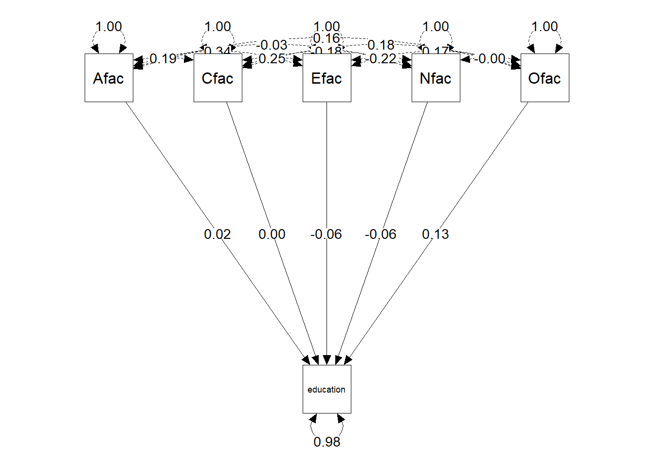
O5 -0.09 0.05 -0.08 -0.10 0.53 0.72 0.28Plotting the standardized multiple regression analysis
The plot shows the standardized partial regression coefficients of the five personality factors (as operationalized by the observed factor scores).
library(semPlot)
semPaths(fit.reg.model,
         ###color       = "black",
         what           = c("std"),
         weighted       = FALSE,
         sizeLat        = 10,
         sizeMan        = 8,
         nCharNodes     = 0,
         edge.label.cex = 1,
         label.cex      = 1,
         edge.color     = "black",
         mar            = c(5,5,5,5))
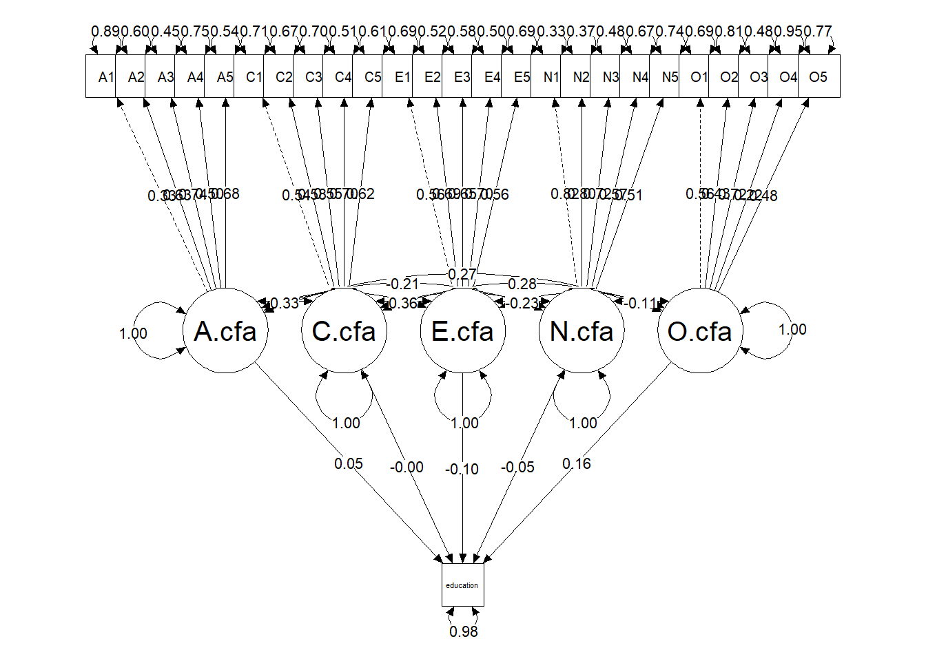
Plotting the standardized sem analysis
The plot of the sem model shows that each personality factor is defined by five items. The plot does not explicitly show it, but each factor is also defined by “what it is not” (i.e. factor loadings that are constrained to zero but not shown in the plot). For instance, the Agreeableness factor is characterised by the five loadings of the Agreeableness items AND the zero loadings of the remaining 20 items. Because this model fit the data poorly we should interpret the parameters with caution.
library(semPlot)
semPaths(fit.sem.model,
         ###color       = "black",
         what           = c("std"),
         weighted       = FALSE,
         sizeLat        = 10,
         sizeMan        = 7,
         nCharNodes     = 0,
         edge.label.cex = 0.8,
         label.cex      = 1,
         edge.color     = "black",
         mar            = c(3,3,3,3))
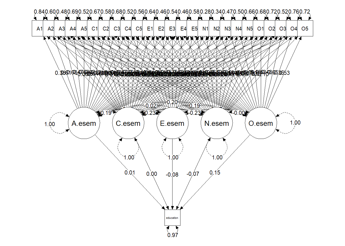
Plotting the standardized esem analysis
The plot of the esem model shows that each factor is loaded by each of the 25 items. The character of each factor is determined by inspecting the pattern of high and low loadings in the standardized factor pattern matrix. The matrix shows that the Agreeableness factor has high loadings (> 0.35) on items A1, A2, A3 A4 and A5. Note that item E4 also has a high loading (0.39). The bulk of the remaining items have relatively low loadings (< 0.15) on the factor.
library(semPlot)
semPaths(fit.esem.model,
         ###color       = "black",
         what           = c("std"),
         weighted       = FALSE,
         sizeLat        = 10,
         sizeMan        = 7,
         nCharNodes     = 0,
         edge.label.cex = 0.8,
         label.cex      = 1,
         edge.color     = "black",
         mar            = c(3,3,3,3))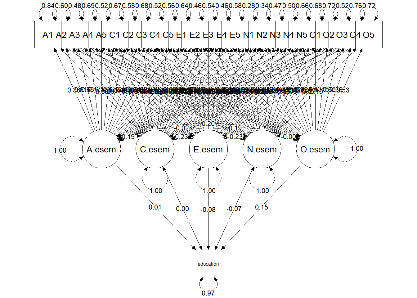
Summary
The multiple regression with observed factor scores, the standard sem analysis and the esem analysis yielded similar results. We can conclude that there is a weak relationship between the big five factors and education. Openness is positively (but weakly) related to education, whereas Extroversion and Neuroticism are negatively (but weakly) related to education. The regression model accounted for about 2% of the variance in education, the sem model for about 2.3%, and the esem model for about 2.8%.